Ideal free distributions form across a regulatory boundary in the Northwest Atlantic Fisheries Organization (NAFO) Division 4X and 5Z groundfish fisheries

Using traditional catch-per-unit-effort (CPUE) indices has resulted in unexpected declines in stock abundance due to lack of sensitivity to conditions such as hyperstability when fishing densely aggregated populations (Rose and Kulka 1999). Estimates derived from CPUE can become unreliable when there is competition and interference between vessels (Gillis and Peterman 1998; Swain and Wade 2003). Efforts to avoid bias from the effects of competition include the use of the ideal free distribution (IFD) (e.g., Swain and Wade 1993). The IFD, first postulated by Fretwell and Lucas (1969). predicts that all individuals will select habitats at which their expectations of fitness will be the highest at equilibrium and at that equilibrium, fitness can not be increased for any individual by means of relocation. Originally used for avian habitat selection, the IFD has been applied to habitat selection research on animals such as gerbils (Makin and Kotler 2019), snowshoe hares (Kawaguchi and Desrochers 2018), and various species of fish (Godin and Keenleyside 1984; Tyler and Gilliam 1995; Shepherd and Litvak 2004), and even outside the field of ecology, anthropologists have used an IFD approach to study past human settlement patterns (Jazwa et al. 2016). IFDs have also emerged in research related to commercial fisheries (Abrahams and Healey 1990; Gillis et al. 1993; Swain and Wade 2003), proving useful when effort distributions that account for interference competition predict underlying fish abundance better than catch per unit effort estimates (Gillis and Peterman 1998; Poos and Rijnsdorp 2007). Methods based on IFDs have also predicted fishing effort distribution and underlying fish abundance when the assumptions of the IFD are violated, including when movement between harvesting locations have costs (Swain and Wade 2003) or around a regulatory closure in a commercial fishery (van der Lee et al. 2014). IFD approaches to commercial fisheries are beneficial due to their simplicity, where the effects of interference and increased exploitation are quantified in a simple equation as a habitat isodar.

The IFD assumes that individuals have perfect information on the expectation of fitness and select the habitat that increases their fitness the most until the system reaches an equilibrium state. It also assumes that individuals are alike and free to move between habitats (Fretwell and Lucas 1969). Conflict may occur between the assumptions of an IFD and the reality of commercial fisheries. Although the IFD assumes that individuals have equal competitive ability across all habitats (Fretwell and Lucas 1969), vessels within a commercial fishery are often not equal competitors, where there may be differences in gross tonnage, length overall (LOA), or engine power (Westrheim and Foucher 1985; Saulthaug and GodØ 2001; Parente 2004). Standardization of catch can be used to equalize fishing power, the ability of a vessel to catch fish (Beverton and Holt 1957), to help meet this assumption. Another problem arises when stocks in different geographical areas are considered distinct for management purposes, even when the underlying populations interact and move across regulatory boundaries (Gullestad et al. 2020).

Morris (1988) developed habitat isodars from the principles of the IFD as equations that demonstrate density levels where fitness is equalized for individuals between multiple habitats in an environment. These isodars provide quantitative and predictive descriptions of IFDs where the details of the underlying resources are not known. A habitat isodar can be portrayed as a series of densities of individuals between two areas such that the expected fitness is equal in each area, meaning the density in one area can be predicted by the density in another area. Isodars have expanded the utility of IFDs in commercial fisheries (Gillis and van der Lee 2012), for instance, being used to predict effort distributions around a regulatory closure (van der Lee et al. 2014).

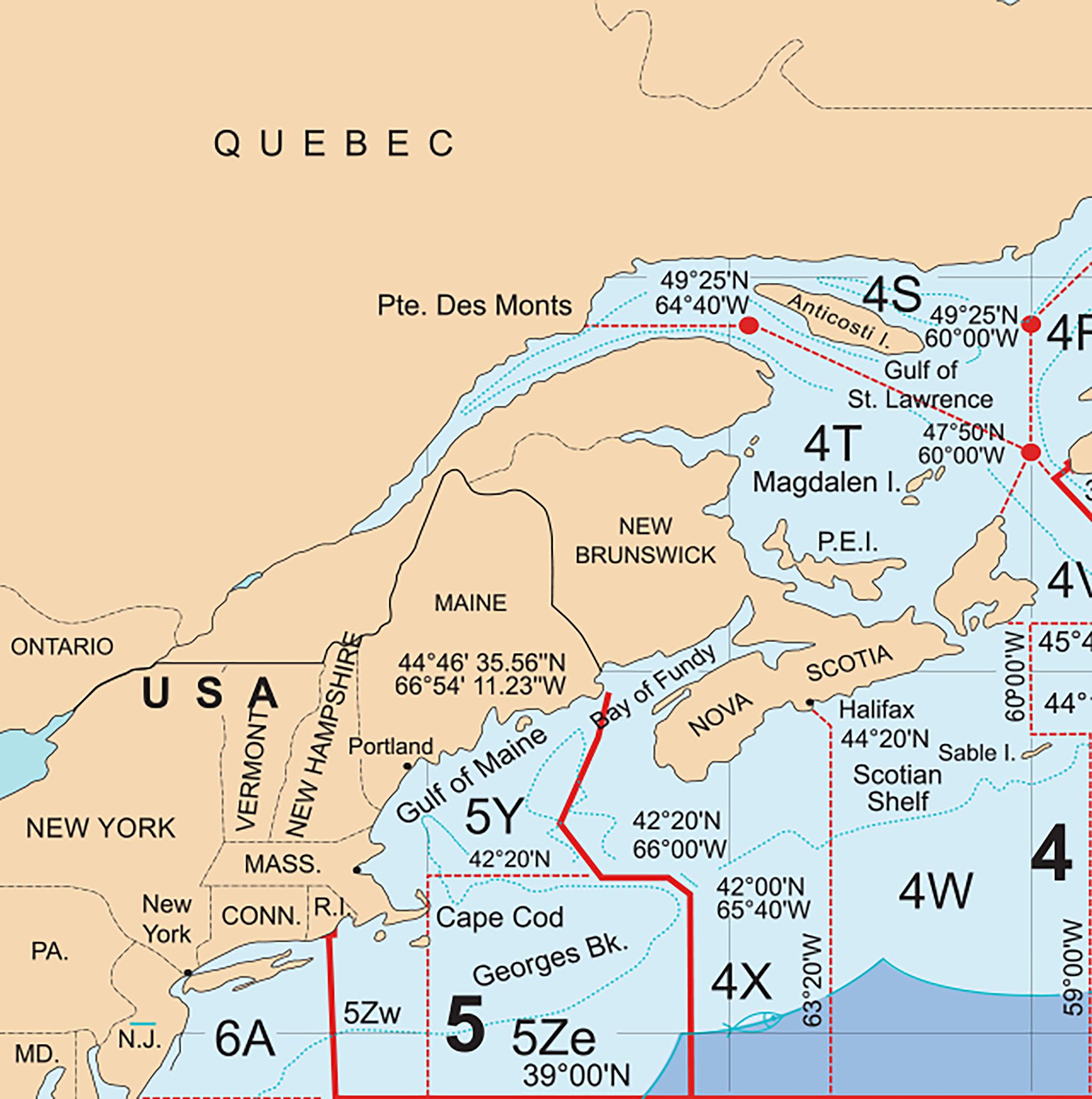
The Northwest Atlantic Fisheries Organization (NAFO) is an intergovernmental body for international cooperation in fisheries science and management that spatially defines regulatory divisions used for fisheries in the western North Atlantic, called the NAFO Convention Area (Northwest Atlantic Fisheries Organization 2024; Fig. 1), wherein Fisheries and Oceans Canada manages commercial fisheries regulations of the Canadian divisions. While IFD research within a regulatory division using isodars exists (van der Lee et al. 2014), it has yet to be seen if an IFD occurs across a regulatory boundary.

We divide NAFO divisions 4X and 5Z into distinct spatial areas based on aggregations of effort within each division by analysing the density of fishing vessels over time throughout both divisions (Enright 2020). We create isodars between these areas to compare the effectiveness of predicting effort in one area based on effort in another area of the same regulatory division against predicting effort using information from an area in a different regulatory division. We do so by standardizing catch data to remove the effects of differences in fishing conditions that could influence catch.

We used logbook data supplied by Fisheries and Oceans Canada from vessels otter trawling for groundfish in NAFO divisions 4X and 5Z from 2005 to 2016 (Fig. 1). NAFO’s 5Z division consists of Georges Bank and is divided internationally between Canada and the United States. The smaller section of 5Z within Canada’s Exclusive Economic Zone together with the entirety of 4X form the area considered in this study. 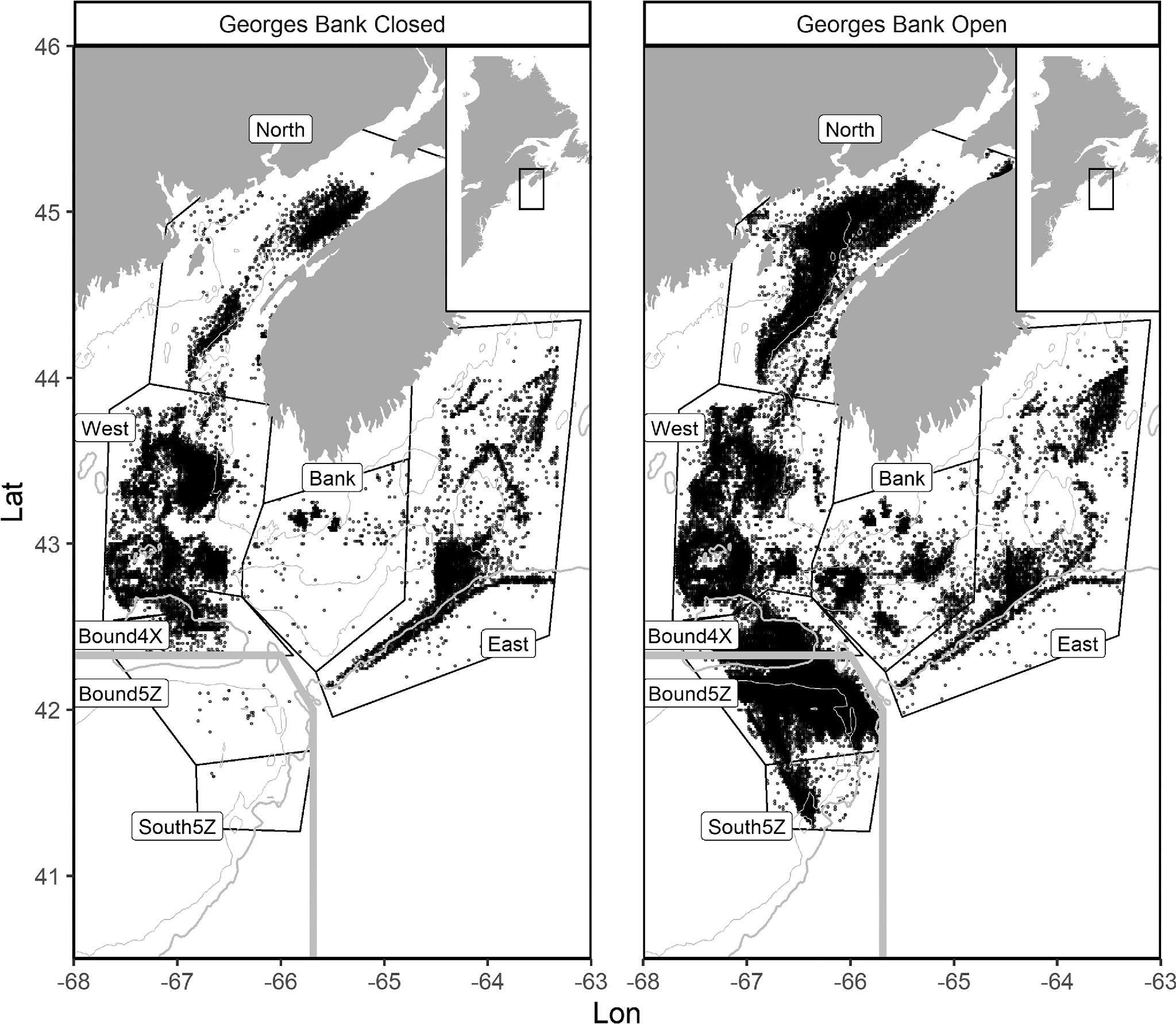Georges Bank has been closed to fishing from 1 March to 31 May annually since 2010, with a variable start date dependent on the spawning condition from previous years (Fisheries and Oceans Canada 2018). Browns Bank within 4X is also under a spawning closure from 1 February to 15 June each year, so fishing effort was only considered when Georges Bank was open, outside of 1 March to 31 May. This excluded the entirety of trawl sets during the Georges Bank closure and most sets during the Browns Bank closure (Fig. 2).

We assigned data into seven discrete geographical areas defined by aggregations of fishing effort within these NAFO divisions with visible gaps separating them from other areas. Areas of low effort concentration were identified and removed using the spatstat library (Baddeley et al. 2015). Set coordinates were placed into a point pattern dataset with the ppp() function. Distances of the nearest sets were determined by the nndist() function. Additional sets that occurred in the same location at different times were excluded to present a more accurate picture of distances between set locations at the same point in time, where otherwise the mean and median distance would be skewed downward when distance between sets in the same location was recorded as zero. We used the density.ppp() function to calculate the expected number of trawl sets that occurred near other sets. Sets in the bottom 10th percentile of these Gaussian kernel-smoothed intensity estimates were removed from the analysis. The standard deviation of the smoothing kernel for the intensity function was the median distance between uniquely-located sets, 1332 m. Under a Gaussian distribution, this standard deviation ensures that most trawl sets that were not removed were conducted further than several times the median distance between sets across the whole area from other trawls; sets in the bottom 10th percentile of intensity were unlikely to be near other sets. This value was large enough to exclude most atypical values and identify aggregations of effort.

One of our effort aggregations spanned the 4X–5Z boundary. We separated this aggregation into two areas divided by their regulatory division to compare isodar predictions across the regulatory boundary. The effort-groupings in 4X are named based on their location within it. North (N4), West (W4), and East (E4) are located in the north, west, and east sections of 4X, respectively. The area in 4X alongside the 4X–5Z boundary called Bound4X (B4), and the area surrounding Browns Bank called Bank (BB) make up the remaining areas of clustered effort in 4X. 5Z is divided into the area alongside the 4X–5Z boundary called Bound5Z (B5) and South5Z (S5), a small separate cluster consisting of the remaining portion of 5Z (Fig. 2).

Catch was converted to a single value for each set, derived from the quantity of each species caught multiplied by the average price per kilogram of each species reported by Fisheries and Oceans Canada (Fisheries and Oceans Canada 2021) in the year it was caught. We divided the catch value of a trawl by hours of effort to obtain value-per-unit-effort (VPUE) as a substitute for CPUE.

There were originally 204 259 sets available for analysis within 4X and 5Z. 112 232 points remained (55% of all data) after removing observations found in one of the following subsets: missing data (4700 points), sets performed by vessels outside of the range of 25 to 150 gross tonnage (36 044 observations) as most observations fell within this range and vessels smaller than the minimum tonnage are unlikely to travel further offshore, sets outside the areas of primary effort concentration (2434 observations), those with no catch value assigned due to the lack of available pricing information (17 071 observations), those reporting clearly inaccurate results, such as sets of a length greater than 7 h (677 observations) or located on land (64 observations), and during the Georges Bank closure (32 480 points).

Fishing effort spread over a large area with vessels individually competing for resources could result in differences between vessels in gear usage and function (Engås and West 1987), vessel size, or decision-making based on distance from the home port (Wilcox and Pomeroy 2003) which could all affect fishing efficiency. We standardized catch value based on a preliminary analysis of the data through a linear mixed model that revealed the variables with the largest impact on VPUE.where V represents value of fish caught, Year is the year fished, and LOA is the length of the vessel performing a set. Variation between individual vessels is represented by a random effect a_j. The residuals, presented in the equation as ε_i, represent differences between predicted and observed catch beyond the influence of year, vessel size, and unique vessel differences. We transformed the residuals back to the original scale by (Y = e^x) so they can be used as standardized catch value in the subsequent analyses.

We present three isodar equations of varying complexity that were originally developed by Gillis and van der Lee (2012); first, the simple classic isodar (IFD; eq. 2), second, the constant productivity ratio (CPR) with common nonlinear effort effects between areas (CPRc; eq. 4), and finally, the constant productivity ratio with unique nonlinear effort effects between areas (CPRu; eq. 6). Each of these isodar equations uses transformed residuals from eq. 1 to represent catch value and hours fished to represent effort so that these isodars are representative of the VPUE in two areas.

The simple classic isodar portrays the isodar described by Morris (1988) where the estimate of mean fitness, catch per unit effort, in one area is equal to that in another. This isodar is represented as the following for two areas:

C_x represents value of catch in area x and f_x represents effort through hours spent fishing in area x. This equation can be rearranged to predict effort in one area based on the catch of both areas and effort in the other area:

The constant productivity ratio isodars expand on this equation, adding the term e^α to represent proportional differences in the cost of fishing between areas, assuming a constant ratio of profitability, and β, which represents nonlinear effects on catch due to changes in effort. A greater α represents the area where effort is being predicted is more desirable than the other area, where a greater β represents increasingly negative effects on CPUE as effort increases. The CPRc isodar, where the nonlinear effects represented by β are common to both habitats, differs from the CPRu isodar, where these nonlinear effects are unique to each habitat. The CPRc isodar is represented as:

This equation can be rearranged to predict effort as well:

The CPRu isodar adjusts the CPRc formula by using a unique β for each area:

This equation can be rearranged to predict effort as well:

The CPRc and CPRu isodars were fit with generalized least squares (a generalized nonlinear least squares model) using the nlme library in R (Pinheiro et al. 2019). Autocorrelation in the residuals of time series is common so we applied several different autoregressive-moving average (ARMA) correlation structures to the GNLS model to identify the α and β parameters of the CPRc and CPRu isodars that provided the best fit. The autoregressive (AR) part of this correlation requires p, the number of correlation parameters in the model. The moving average (MA) correlation requires q, the number of noise terms included in the correlation structure. Together, p represents correlation parameters and q represents noise terms to account for correlation with previous observations. The ARMA model benefits from its capacity for requiring fewer parameters compared to an autoregressive model alone (Box et al. 2015). Different combinations of p and q were used for the ARMA model with a minimum p of 1 and maximum p of 3, and a minimum q of 0 and maximum q of 3 to ensure p + q < p’, the p term used in a simple AR model used for comparison. We used the corrected Akaike information criterion (AICc; Hurvich and Tsai 1989) for model selection to determine which combination of the p and q parameters resulted in the GNLSmodel that minimized data loss while best explaining variation, helping us quantify the CPRc and CPRu isodar parameters. The results from the isodar with the chosen parameters represent the predicted amount of effort in an area.

We used weekly aggregations (108 weeks where fishing occurred from January 2005 to December 2016, after initial data removals) of catch value and effort as a time series of data for each of the three types of isodars. Each isodar used these time series data from a pair of the subdivided areas within 4X or 5Z: an area within either 4X or 5Z paired with the area on the boundary of each division, or two areas on opposing sides of the boundary, for a total of eleven pair combinations to examine with isodars. Each isodar used effort in one area as a parameter to predict effort in the opposite area using one of eqs. 3, 5, and 7. We used a standard major axis regression on the results of weekly effort predicted by the isodars against observed effort in the same time period to examine the effectiveness of each isodar. Model II regressions, such as standard major axis regressions, are used when the independent variable in the model is not controlled, and error is present on both axes. The regression line in standard major axis regressions is calculated by minimizing the area of the triangle formed between the plotted points and the regression line, where the three points are the point of observed and predicted effort and the horizontal and vertical axis values on the regression line that align with the respective coordinates of the effort value (Legendre and Legendre 2012). The slope and correlation coefficient of each model, using Model II errors, were found using the smatr library in R (Warton et al. 2012). Isodars were considered to be an accurate effort predictor when the confidence interval of the regression slope for predicted effort against observed effort contained 1.

The best standardization model used year, LOA, and a random effect of vessel IDs to represent variation between unique vessels (Marginal R² = 0.11, Conditional R² = 0.23). After standardization, much variation remained to be examined with isodars. The value of the α parameters varied between isodars predicting effort across the regulatory boundary. The full range of the α confidence intervals for each isodar that accurately predicted effort in Bound5Z was above 0 except for W->B5, which was 0 (Table 1). A value above 0 indicates that predicted effort is expected to be greater than observed effort in the other area. The effect of increasing effort was represented by β in the isodar equation. A value greater than one represents negative effects related to competition in the fishery that increase nonlinearly as effort increases. Each β in 5Z is greater than one, whereas the majority of β values in 4X are around 1 (Table 1), indicating that these negative density-dependent effects are occurring in 5Z.

The greater β in 5Z compared to 4X reflects how the high density of trawling activity in Bound5Z increases the costs of fishing (Table 2). West was the only area with a corresponding β value greater than that of Bound5Z. West also has the greatest set density (Table 2). β appears to be related to density but the trend is inconsistent. It may be more accurate to consider β as related to the size of each area instead, as negative impacts from competition in these smaller areas increase exponentially as effort increases (β > 1), whereas the larger areas tend to lack these any effect caused by increased effort (β = 1).

Isodars show varying success at predicting effort accurately. Based on the predicted-on-observed regression’s slope, the simple isodar, representing the classic IFD, demonstrated the lowest accuracy with only two out of eleven area pairings in which the isodar accurately predicted effort (Slope ≈ 1) in one area based on effort in the other area. The CPRc isodar was able to accurately predict effort in seven of the eleven area pairings. The most complex isodar, the CPRu isodar, was accurate seven out of eleven times as well, and was the only isodar to predict effort accurately between Bound4X and Bound5Z (Table 3). The following analyses focus on successful CPRu isodars, with the addition of examining violations to ideal free assumptions to gather insight into the reason why some isodars were unsuccessful.

Although the presence of a regulatory boundary goes against the assumption of free movement in IFDs, the majority of CPRu isodars predicting effort from 4X to 5Z were still accurate, including the B4->B5 isodar (Table 3). Of the 94 unique vessels that fished in 4X and 5Z during the study period, 78 fished in both divisions and none fished only in 5Z. All CPRu isodars predicting effort in South using effort from areas within 4X were accurate. However, only W4->B5 and B4->B5 were successful among isodars predicting effort in Bound5Z. These isodars notably performed better than the isodar consisting of both sub-areas within 5Z, S5->B5 (Table 3).

Our isodars demonstrate that effort on one side of the NAFO 4X–5Z boundary is related to fishing success on the other side of the boundary, and missing catch or effort values from either side can be predicted by the remaining values. The results confirm that isodars can predict effort (Gillis and van der Lee 2012), even when a regulatory boundary exists between the two areas of focus. The complicated nature of these fisheries dynamics requires additional complexity to more closely represent real world conditions, as demonstrated by the relative success of the CPRu isodar compared to the CPRc or simple classic isodars. The accuracy of the CPRu isodar is due to the additional parameters that account for travel costs and other unique costs of fishing in each area. Accurate effort prediction across the regulatory boundary is a novel finding that demonstrates the need to consider the interdependence of divisions and how neighbouring regulatory divisions can influence fisheries management outcomes.

Gillis and van der Lee (2012) furthered the isodar approach to use in commercial fisheries by developing models with parameters that represent unknown costs due to competition. The addition of 5Z to the analysis builds on this work by expanding the area of focus to include 5Z, an adjacent regulatory division that was accessible to many of the same vessels fishing in 4X in their study. The isodars defined by Gillis and van der Lee (2012) could have been affected unexpectedly when fleets incorporate 5Z into their decision making when choosing where to fish. Isodars were able to predict effort across the 4X–5Z boundary in many cases, even while some isodars were unable to predict effort in parts of 5Z using catch information from other parts of 5Z. A notable reduction in effort near the 4X–5Z boundary in winter provides an example of the variability present in these data, where unstable weather and unpredictable catch rates discourage traveling far (P. Comeau, personal communications, 2019). The cross-boundary nature of this fishery responds through increased fishing in areas closer to home ports in Nova Scotia.

Although regulations on commercial fisheries limited movement across the boundary, breaking one of the assumptions of the IFD (Fretwell and Lucas 1969), all effort in 5Z came from vessels that were also able to fish in 4X at some point during the study period. The ability to fish on both sides of the regulatory boundary by many vessels may have reduced the effects of violating the classic assumption of free movement, especially between Bound4X and Bound5Z. This finding suggests that completely free movement is not necessary for local catch rates to reflect fishing success in neighbouring areas in this fishery, and at a broader scale the predictions that arise from theories of habitat selection. Although the more complicated isodars account for differences in the cost of foraging between areas, the simple isodar representing the classic IFD still predicted effort accurately in B5 using information from N4 and W4. Violations to other assumptions of the IFD do not always restrict the formation of IFDs. Unequal competitive abilities can result in a distribution still resembling an IFD of equal competitors (Hugie and Grand 1998; Smallegange and van der Meer 2009). Even when the assumption of ideal knowledge is broken and individuals move suboptimally, as long as they can identify the payoff of foraging in their current location as greater than other areas, the population will still converge toward an IFD (Cressman and Křivan 2006).

The accuracy of isodars predicting effort in Bound5Z from effort in West and Bound4X, the two nearest areas within 4X to Bound5Z, demonstrates that fishers in these nearby areas may have better information on fishing success in Bound5Z in contrast to those fishing in more distant areas. While ideal knowledge is not mandatory for local effort to reflect success in neighbouring areas (Cressman and Křivan 2006), this is less likely to occur when information is imperfect (Matsumura et al. 2010). The failure of the S5->B5 isodar to predict effort accurately within the same regulatory division as opposed to these two isodars across a regulatory boundary provides further evidence that local catch and effort distributions are linked across this regulatory boundary.

The predictive isodars in this fishery support the consideration of IFDs and related effort distributions in studies involving human harvest. IFDs may arise so frequently because individuals maximize their fitness across multiple patches of resources in the environment, to the point where natural selection favours dispersal strategies that form them over alternative strategies (Cantrell et al. 2017). This strategy may be naturally favoured to the point that species that do not meet some of the assumptions of the IFD can still form one (Griffen 2009); similarly, we demonstrate that the distribution of fishing vessels resembles this strategy across a regulatory boundary through our habitat isodars. Fisheries managers should then consider vessel movement across regulatory boundaries in addition to the known impact of increasingly negative impacts on fishing success from greater competition when predicting stock abundance through the use of catch rates (Swain and Wade 2003; Poos and Rijnsdorp 2007). Effort distributions can reveal the underlying movements of fish by matching their distribution to maximize fishing success through the same principles as the IFD. Fish are not bound to one regulatory division, and fish harvesters may find a neighbouring regulatory division attractive when they have licenses for both areas. While previous work has found CPUE can be less reliable than effort distributions (Swain and Wade 2003), violations of the assumptions of the IFD were to blame. Isodars can advance fisheries modelling by taking these violations into the model; our isodars successfully predicted effort across a regulatory boundary where the assumption of free movement is violated. Therefore, more reliable indices of relative abundance can be obtained from isodars when the factors that impact catch are understood and accounted for in these estimates, such as through the examination of cross-boundary distributions and differences in local competition levels. Isodars can then reveal how much of the local variation in catch is due to differences in fish abundance rather than differences in the ease of catchability through the understanding that the distribution of vessels matches the underlying distribution of fish.