Open access

Spatial and seasonal determinants of arthropod community composition across an agro-ecosystem landscape

Publication: FACETS
8 November 2024

Abstract

We used Malaise traps to sample arthropod community composition at biweekly intervals across an agroecosystem landscape in southern Ontario, Canada, to evaluate the relative impact of site spacing, seasonal timing, weather conditions, local plant community attributes, and agricultural extent across the local landscape on spatial and temporal variation in arthropod community composition. The 15 field sites sampled spanned a wide gradient of agricultural extent that in isolation had a strong impact on spatial variation in arthropod community composition. DNA metabarcoding of the samples identified >10 000 different arthropod biodiversity index numbers. Local variation in plant community composition and canopy cover best explained variation in arthropod community dissimilarity. Weather variables followed closely in explanatory power, driven primarily by seasonal variation in temperature. Significant effects of time remained after accounting for environmental variables, with little independent effect of spatial distance. The proportion of agricultural land at the landscape scale had little detectable effect after controlling for the influence of the other environmental variables. Our results suggest that plant community composition, cover, weather conditions, and seasonality structured the arthropod community to considerable degree.

Introduction

Rapid declines in arthropod abundance and species diversity across the globe have received a great deal of recent attention (Gossner et al. 2016; Hallmann et al. 2017; Sánchez-Bayo and Wyckhuys 2019; Seibold et al. 2019; Wagner et al. 2021). These drastic changes in arthropod communities are a major cause for concern, given their enormous taxonomic and functional diversity and critical role in the provisioning of vital ecological services such as pollination, pest control, and nutrient cycling (Kremen et al. 1993; Stork 2018). Although the causes of arthropod declines are surely complex and multi-faceted, habitat loss and external inputs associated with agriculture are frequently identified as primary drivers (Gossner et al. 2016; Sánchez-Bayo and Wyckhuys 2019; Seibold et al. 2019; Wagner 2020). Recent work suggests, however, that arthropod declines are not universal (Crossley et al. 2020; van Klink et al. 2020), raising fundamental questions about the regulation of arthropod biodiversity in agroecosystems (Wagner 2020).
Agroecosystems contain a mosaic of crop and non-crop habitat, the balance of which is an important determinant of arthropod biodiversity as non-crop habitat provides a spatiotemporally stable source of food, shelter, nesting, and mating resources (Dolezal et al. 2022). Specifically, variation in arthropod community composition has been linked to local attributes, including plant biomass, structural complexity, and plant community composition (Stinson and Brown 1983; Schaffers et al. 2008; Borer et al. 2012; Prather and Kaspari 2019) as well as landscape-level measures of habitat diversity, land-use intensity, landscape connectivity, and landscape complexity (Schweiger et al. 2005; Hendrickx et al. 2007; Fahrig et al. 2011; Gossner et al. 2016; Seibold et al. 2019). Compositional differences in arthropod communities may also result from dispersal limitation and ecological drift, effects of which are often exacerbated by patch isolation and especially affect groups with limited dispersal ability (Bell 2001; Hubbell 2001; Vellend 2010). This is significant since many arthropod taxa have rapid generation times and thus the influences of temporal and spatial processes on community divergence can be powerful even within a single growing season (Kingsolver 1989; Chown and Gaston 1999). Given the paucity of non-crop habitat in many agroecosystems, measures aimed at maintaining and restoring natural areas can be very effective in promoting arthropod biodiversity (Paterson et al. 2019; Dolezal et al. 2022). Several studies have demonstrated that restored habitat can lead to an increase in arthropod richness and abundance, often with positive effects on ecosystem services such as herbivore suppression, pollination, and predation services (Albrecht et al. 2020; Paterson et al. 2019; Dolezal et al. 2022).
Most of these community-shaping processes have been investigated from a spatial perspective, but temporal factors can also play a central role (Grøtan et al. 2012). Seasonality is particularly important in many systems, stemming from an interplay of species-specific responses to abiotic conditions, such as temperature and precipitation, biotic conditions, such as plant resource availability, and stochastic variation through time (Wolda 1978, 1988; Stinson and Brown 1983; Grøtan et al. 2012; Hatosy et al. 2013). Previous studies have found that the effect of habitat composition and the configuration of those habitats in the landscape on arthropod communities can vary across the growing season (Bertrand et al. 2016) and that landscape composition can modulate phenological diversity (Sydenham et al. 2014). Even in tropical systems with less pronounced seasonality compared to temperate regions, arthropod community composition in both natural forests and rubber plantations shows high seasonal turnover (Beng et al. 2018). Arthropods living in agroecosystems experience both seasonal climatic variation and season-dependent management actions such as plowing, planting, and pesticide application (Anderson et al. 2012; Beckmann et al. 2019; Hausmann et al. 2019).
Based on these previous studies, our primary goal was to evaluate the relative impact of local, landscape, and seasonal variables for explaining variation in arthropod community composition across a highly heterogeneous agroecosystem landscape that varies in the coverage of dedicated cropland and native habitats. Our secondary goal was to evaluate the utility of metabarcoding of Malaise trap samples as a simple and repeatable means of monitoring arthropod biodiversity. Our third goal was to establish an arthropod biodiversity benchmark that spans a wide gradient of land use types by which the effectiveness of land restoration activities on the ALUS farm network might be evaluated in future years.
On the basis of the extensive body of insect community research described above, we predicted a positive relationship between arthropod community dissimilarity and environmental distances. That is, larger differences in environmental conditions should generate more dissimilar communities for environmental variables representing weather, plant community attributes, or agricultural extent across the landscape. To account for possible effects of dispersal limitation, ecological drift, and/or unquantified spatiotemporally structured environmental variables, we incorporated a novel framework proposed by Jabot et al. (2020) for linking spatial and temporal distances as covariates in analyses with environmental variables.

Methods

Study sites

In late April/early May 2019, 29 Townes style Malaise traps were placed at 12 farms and 3 conservation areas in Southern Ontario, Canada (Fig. 1), with field sites separated on average by 49 km (range = 7–142 km, sd = 31 km). Nine of the 12 farms sampled were part of the ALUS program, designed to fund restoration of prairie or wetland habitats in marginally productive cropland. Study site locations were chosen opportunistically. While the sites chosen clearly span a wide range of land uses, no effort was made to ensure that the sites selected for this study are representative of the entire region. Most of the study region is heavily farmed with crop monocultures typically of corn (Zea mays), soybean (Glycine max), and winter wheat (Triticum aestivum) covering ∼90% of the landscape. The remaining 10% of the landscape is largely composed of a heterogeneous mixture of wetlands, woodlots, and riverine margins (Fig. 1). Mean annual temperatures are 8 °C, with precipitation averaging 1035.8 mm (http://climate.weather.gc.ca).
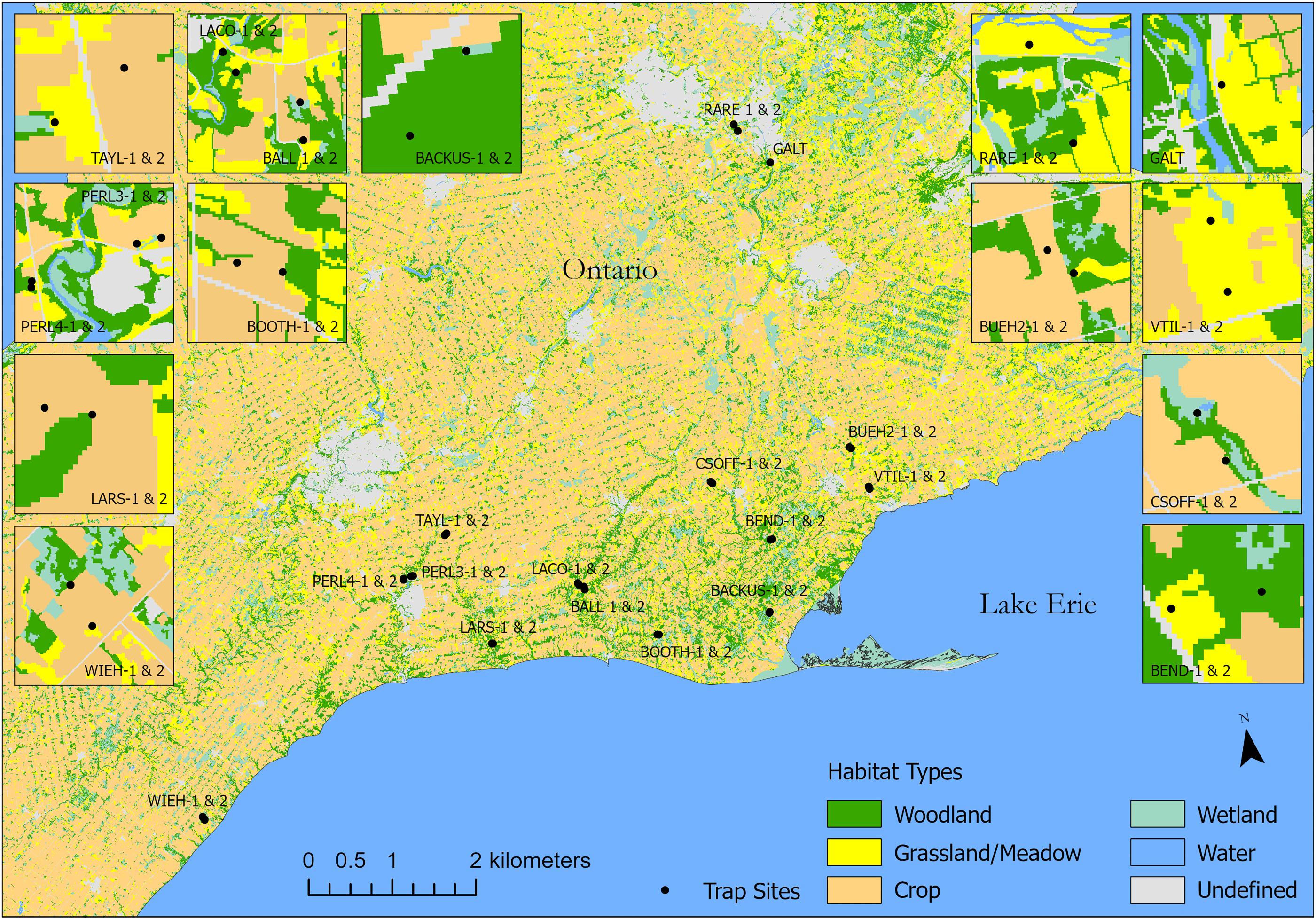
Fig. 1.
Fig. 1. Map of the study sites in southern Ontario. Landcover data were obtained from the 2019 Annual Crop Inventory, which classifies landcover types from satellite images with 30 m spatial resolution using decision tree algorithms (Agriculture and Agri-Food Canada 2020). Mapping is based on a Lambert projection with longitude/latitude coordinate system.
With the exception of one site that only had one trap, two traps were placed per farm or conservation area, with traps specifically placed on the same farm or conservation area separated by 371 m on average (sd = 282 m) (Fig. 1). Malaise traps are well suited for large-scale monitoring as they are easily standardized, time and cost effective, and sample a wide array of arthropod taxa, though they preferentially trap flying insects (D'Souza and Hebert 2018; deWaard et al. 2019). The placement of Malaise traps on the sites sampled four crude habitat types in varying proportions: woodland, grassland/meadow, wetland, and cropland. All of the farms and conservation areas in our study had at least three, and some had four of these crude habitat types (Fig. 1). Trap placement locations were chosen to ensure that at least two habitats were sampled within a given farm or conservation area while maintaining a relatively balanced (albeit imperfectly balanced) representation of habitat features across the full set of 19 farms and conservation areas. Due to the heterogeneous mixture of habitats on the farms and conservation areas, many traps were placed within 100 m of the edge between habitat types (Fig. 1).
Preliminary modelling of path analysis indicated that crude habitat designations were far less useful in explaining variation in arthropod community composition than a set of continuous floristic features (richness, cover, canopy height, and floristic composition). In the interests of parsimony, we accordingly dropped habitat type from subsequent path analyses.

Arthropod data

Arthropods were collected in 500 mL plastic bottles filled with 90% ethanol (Thermo Fisher Scientific A962P-4) attached to the trap heads. The bottles were collected and replaced biweekly from May through mid-October 2019. With few exceptions (damaged samples or early trap takedown), 12 two-week samples were collected at each trap, with one trap set per site. All of the collected samples were accessioned and are stored at the Centre for Biodiversity Genomics (CBG) (https://biodiversitygenomics.net). Every other 2-week sample was sent for DNA metabarcoding at the CBG’s sequencing facility (https://ccdb.ca/).
The metabarcoding analysis targeted a 462 bp amplicon of the mitochondrial cytochrome c oxidase subunit I gene which was polymerase chain reaction amplified from the DNA of each bulk sample using the forward primer AncientLepF3 (Prosser et al. 2016) and the reverse primer cocktail C_LepFo1R (containing LepR1 and HCO2198) (Hebert et al. 2004). This primer set has demonstrated effectiveness in recovering the barcode region across the wide diversity of arthropods regularly collected by Malaise traps. In addition, the amplicon it generates is sufficiently long to provide solid taxonomic resolution while still short enough for the size limitations imposed by high throughput sequencing systems such as the Ion Torrent S5 platform (Thermo Fisher Scientific) used here (Braukmann et al. 2019). Detailed laboratory methods are provided in supplementary information (SI). Sequences recovered from eight replicates from each of the 172 samples were uploaded to the mBRAVE platform (Ratnasingham 2019; https://www.mbrave.net/) where they underwent several analytical steps (see protocols described in SI) required to allow their assignment to a Barcode Index Number (BIN) that serves as a species proxy (Ratnasingham and Hebert 2013) based on queries between sequences and reference libraries for chordates, insects, non-insect arthropods, non-arthropod invertebrates, and bacteria. BIN assignments and the taxonomic assignments associated with them are dynamic because they are impacted by the continual expansion of sequence records on Biodiversity Of Life Database (BOLD). The taxonomic assignments reported in this study are those current in November 2019. Only arthropods and non-arthropod invertebrates were included in the final BIN table, although arthropods constituted 99.8% of these BINs.
The Centre for Biodiversity Genomics at the University of Guelph has a separate archive for analyzed bulk trap samples such as the metabarcoded Malaise trap samples from this study. Each sample is lysed in its bottle, aliquots are taken for DNA extraction, then the lysate is filtered off, and fresh ethanol is added back to the bottle before archiving. Because of this non-destructive extraction method, the specimens within the sample bottles are intact and available for loan and/or further study. The individual specimens have not been removed, sorted or pinned (but they can be by subsequent researchers), and all the sample bottles are catalogued in our collection for easy retrieval.

Plant community attributes

Floristic surveys of ground vegetation were conducted monthly on a four-week rotating schedule between May and September, given the importance of non-crop plant resources for food, shelter, and nesting for many arthropods of farm landscapes. Two plant survey techniques were used over the course of the sampling period. For the first three weeks, five quadrats measuring 1x1 m were randomly placed on each side within 25 m of the Malaise trap for a total of ten quadrats per trap. To simplify the process of quadrat placement, we thereafter placed quadrats at 5 m intervals along two transects oriented away from the trap. 1 m × 1 m quadrats were placed every 5 m along the transects, for a total of 10 quadrats per trap. For traps that had been placed within 100 m of habitat boundaries, plant transects were oriented orthogonally to the habitat edge.
The identity and percent cover of each plant as well as overhead canopy openness were measured in each plot. Overhead canopy openness was measured given the importance of canopy on microclimate, to which ectothermic arthropods can be highly sensitive. Openness was determined using a convex spherical densiometer (Forestry Suppliers), averaged from four points perpendicular to each side of each plot. Only canopy openness from the second set of plant surveys was used in the analyses as tall vegetation could obscure canopy measurements in later months. Given some uncertainty about field identification of closely related forbs and grasses that were not in flower, all plant data were analysed at the genus level or higher. Because of uncertainty in the identification of some non-native C3 pasture grasses (e.g., Poa or Festuca), some of these grasses were classified into the tribe Festuceae.

Weather data

Given that arthropods can be influenced by weather conditions either via physiological mechanisms or by influences on dispersal, weather data were sourced from the Government of Canada Historical Weather Database (https://climate.weather.gc.ca/) from five weather stations closest to the sampling sites as well as temperature loggers attached to each Malaise trap. The loggers recorded temperature (°C) hourly throughout the entire sampling period for each trap. Six loggers malfunctioned; in these cases, temperature data were taken from another trap on the same farm (five traps) or from the nearest site (one trap due to a logger malfunction in the only trap at the site). Hourly relative humidity (%), hourly wind direction (10 s deg), and hourly wind speed (km/h) were obtained from four weather stations. Total daily precipitation (mm) was only available for three stations, so in one case these data were taken from another nearby station. All variables were averaged, and the coefficient of variation was calculated for the temperature data to match the two-week sampling periods of the nearest traps throughout the season. Since the weather variables were expected to be correlated, principal components analysis (PCA) was used to extract the main axes of variation before analysis. Four axes were retained, representing 88% of the total variation.

Landcover data

Landcover data were obtained from the 2019 Annual Crop Inventory, which classifies landcover types from satellite images with 30 m spatial resolution using decision tree algorithms (Agriculture and Agri-Food Canada 2020). All landcover types were reclassified into cropland (excluding pasture/forage and fallow land), semi-natural, and urban categories prior to analysis. Since the percentages of semi-natural and agricultural land were highly correlated and we were primarily interested in the impact of agricultural extent across the local landscape, only the percentage of the landscape that is agricultural within a 2000 m radius was used in the analysis. This radius extends beyond the boundary of the farms and conservation areas we sampled. This scale better represents landscape-level processes including dispersal limitation and spatial turnover in habitat quality, with strong effects of landscape factors on arthropods at 1000–2000 m scales previously observed (Gámez-Virués et al. 2015; Siebold et al. 2019). These metrics were calculated using the landscapemetrics R package (Hesselbarth et al. 2019). In the best of worlds, one would hope to incorporate local farming practices into such an analysis to characterize agricultural extent as well as spatial extent. Due to privacy concerns, however, we did not have access to crucial information on farming practices, such as the level and frequency of pesticide and fertilizer application. We accordingly did not include local metrics of agricultural intensity in our analysis.

Statistical methods

To explore general patterns of spatiotemporal β diversity, a dissimilarity approach based on the Sørensen index was taken where arthropods were grouped by trap across all time periods, by time period across all traps, and for all samples. In the first case, there were 29 units for comparison (traps), in the second there were 6 (time periods) and in the third there were 172 (samples; trap by time combinations). Since the temporal extent of the arthropod and plant data differed slightly (6 months and 5 months, respectively), the arthropod data were filtered to the samples that were closest in time to the plant data for all analyses that involve environmental effects. This meant that either the first arthropod sample or the last arthropod sample was omitted, depending on the plant survey schedule. This left 144 samples available for analysis.
We conducted a distance-based path analysis based on the framework proposed by Jabot et al. (2020) using modified scripts from those provided in their supplementary material. These scripts use the “SEM” function in the R package lavaan to fit the path analysis model (Rosseel 2012). The structure of the path model was as follows: arthropod Sørensen dissimilarities between samples were linked to eight environmental distance variables. Three represented plant community attributes, one represented agricultural extent across the local landscape, and four represented weather variation (see Table 1 for a full list). Based on hypothesized relationships between the plant community attributes, plant richness and canopy cover were allowed to have both a direct effect on arthropod community (Sørensen) dissimilarity as well as an indirect effect through plant community composition. Arthropod Sørensen dissimilarities were directly linked to spatial and temporal distances, and each environmental distance was also linked with spatial and/or temporal distance depending on whether it showed spatial variation, temporal variation, or both (Table 1). Environmental distances were calculated as Euclidian distances except for differences in plant communities, which were calculated as Bray–Curtis dissimilarities of the plant cover data. Spatial distances were calculated as the distance in meters between individual traps using latitude/longitude coordinates and the geodist R package (Padgham and Sumner 2020). Given that field sites were >2 orders of magnitude farther apart (mean = 49 000 m) than were those on a given farm or conservation area (mean = 371 m), distance also serves as a reliable statistical proxy for farm identity. Temporal distances were calculated as the Euclidian distance between sampling periods (e.g., the distance between sampling period 1 and 6 would be 5, referring to a difference in time of ∼5 months).
Table 1.
Table 1. Environmental variables considered in the path analysis and their groupings into either plant community attributes, agricultural extent, or climatic variables.
GroupVariableType of variation
Plant communityCanopy opennessS
AttributesPlant genus richnessS + T
 Bray-curtis plant community compositionS + T
Agricultural extent% Agriculture in 2KM radiusS
ClimaticAverage temperatureS + T
 Average relative humidityS + T*
 CV temperatureS + T
 Average wind speedS + T*
 Average wind directionS + T*
 Average precipitationS + T*

Note: Type of variation indicates whether the explanatory variable exhibits spatial (S) temporal (T) or spatiotemporal (S + T) variation.

*Limited spatial variation based on closest weather stations. Climatic variables were subject to principal components analysis prior to use in path analysis and 4 axes were retained, explaining 88% of the variation.

The importance of each significant path in the model was assessed based on standardized path coefficients (SPCs). Model fit was assessed based on a combination of the standardized root mean square residual index (SRMR), the root mean square error of approximation index (RMSEA), and the comparative fit index (CFI). Values typically indicating acceptable to perfect model fit for each index range between 0.09–0, 0.08–0, and 0.90–1, respectively (McDonald and Ho 2002; Fan et al. 2016). Since the independence assumption of path analysis would be otherwise violated by using pairwise dissimilarity values, the significance of parameters was determined using the permutation method of Fourtune et al. (2018). This was also done using scripts provided by Jabot et al. (2020) and the R package MASS was used in the permutation procedure (Venables and Ripley 2002). The Benjamini–Hochberg procedure was used to correct P values for multiple comparisons (Benjamini and Hochberg 1995; Jabot et al. 2020). Values of paths to and from groups of environmental distances were calculated by summing the absolute values of significant SPCs of individual environmental variables, including both direct and indirect effects (Jabot et al. 2020). We additionally used a variance partitioning approach based on multiple regression (Tuomisto et al. 2012) to investigate the unique explanatory power of time and space while controlling for environmental variation and vice versa. Analyses were carried out using R statistical software version 3.6.3 (R Core Team 2020) at a significance level of α = 0.05.

Results

Patterns of arthropod biodiversity

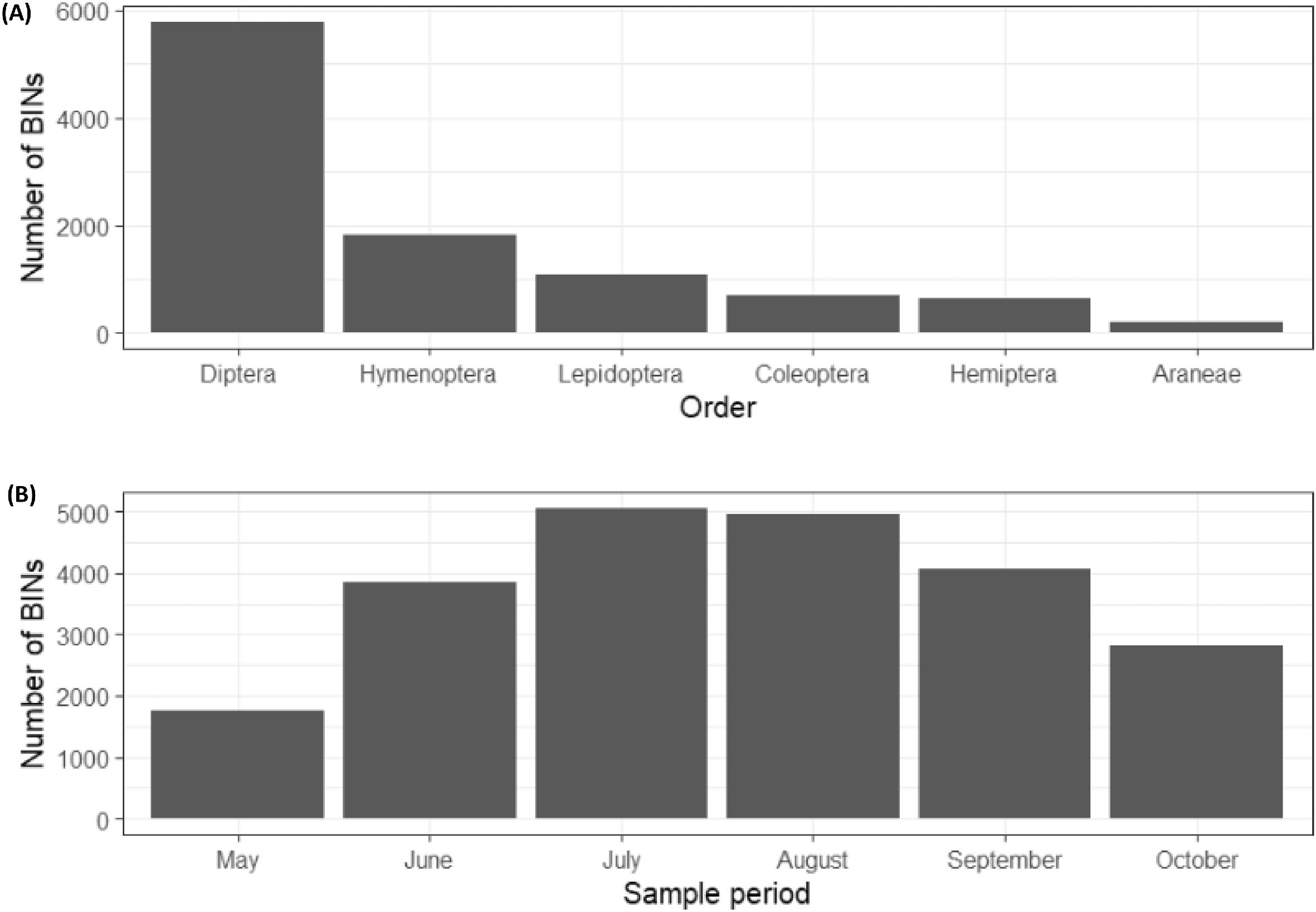
The number of different BINs arising from the arthropods collected per Malaise trap over a two-week period varied strongly among samples (mean = 347, sd = 151; range = 51–792). The greatest number of BINs identified from a single trap over the course of the season was 1851 while the lowest was 983, and the average was 1335. Many BINs were uncommon with 39% of BINs represented by only a single occurrence. 53% of BINs belonged to the order Diptera, 17% to Hymenoptera, 10% to Lepidoptera, 6% to Coleoptera, 6% to Hemiptera, and 2% to Araneae (Fig. 2A). A total of 144 samples had temporally matching arthropod and plant samples available for analysis. Among this total, 10 359 BINs were identified, with representatives from 34 orders and 428 families, including 3777 known species in the BOLD database. Arthropod diversity was highest in July with 5059 BINs and lowest in May with just a total of 1761 BINs (Fig. 2B). The average number of BINs per sampling period was 3748.
Fig. 2.
Fig. 2. Distribution of arthropod BINs (Barcode Index Number; a species proxy) for (A) the top six most species-rich orders of arthropods across all samples and (B) among sample periods pooled across all traps.
Arthropod Sorensen dissimilarity among traps across all time periods was very high (mean = 0.73, sd = 0.09), as was dissimilarity among time periods across all traps (mean = 0.61, sd = 0.12). The highest pairwise dissimilarity among months was 0.80, involving comparisons between May and August, while the lowest was 0.44, both between July and August and between August and September.
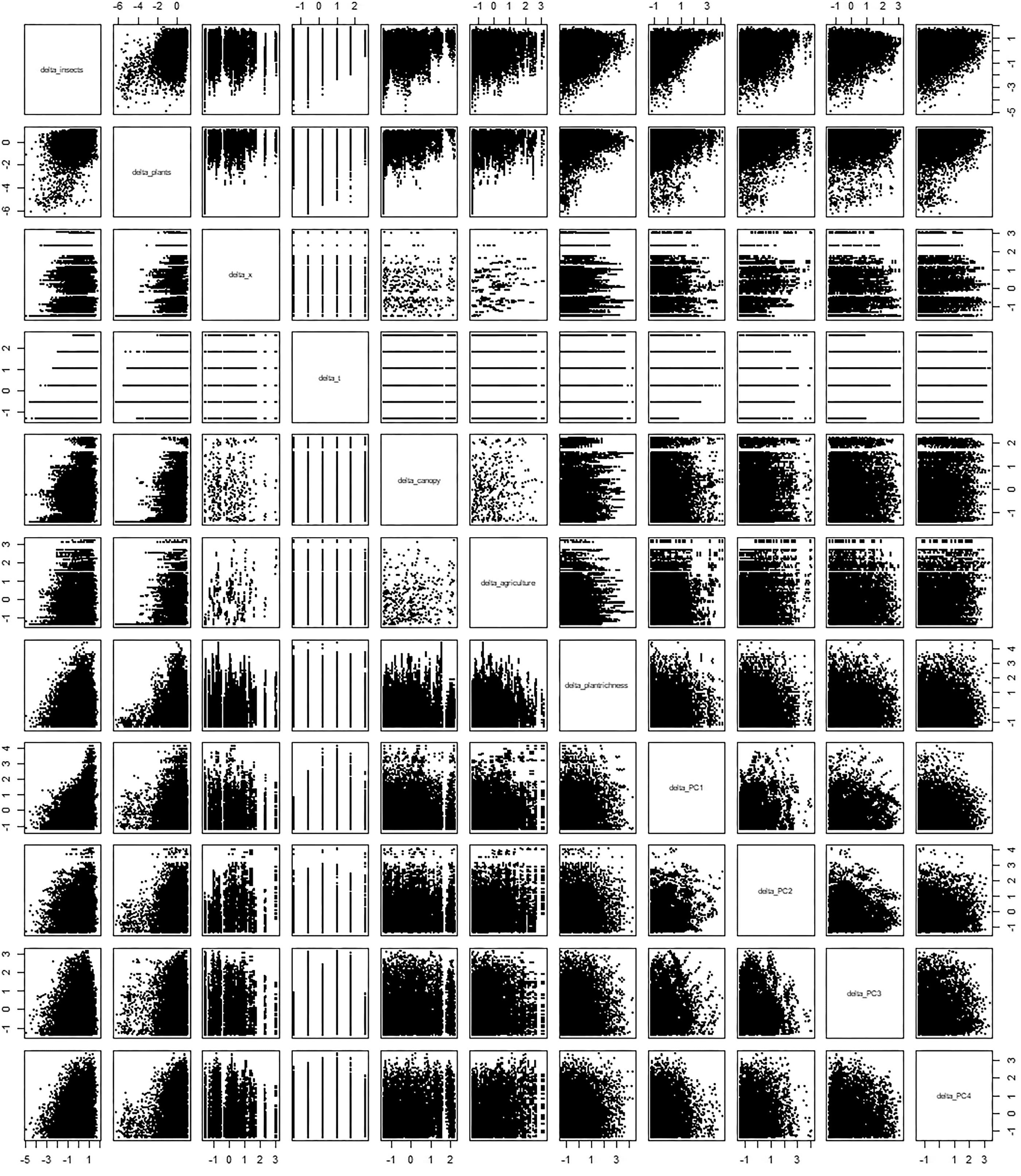
Variation in arthropod community composition among trap sites was strongly related to local agricultural extent (F1,10294 = 2395, P < 0.001, R2 = 0.188), such that traps in locales with a similar agricultural footprint tended to be more similar in species composition than traps with widely differing agricultural footprint (Fig. 3). Not surprisingly for a dataset of this magnitude of replication (6 sample dates × 29 sites), however, every variable was shaped to some degree by the other variables in the dataset (Fig. 4), suggesting the need for path analysis to partition covariation across environmental correlates (Shipley 2016). Both arthropod community dissimilarity and plant community dissimilarity shared particularly strong patterns of covariation with almost every other variable in our dataset (rows A and B in Fig. 4).
Fig. 3.
Fig. 3. Variation in arthropod community composition in relation to variation in agricultural extent.
Fig. 4.
Fig. 4. Scatter-plots of all standardized variables used in the structural equation models (A = Δ arthropod community, B = Δ plant community, C = Δ space, D = Δ time, E = Δ canopy cover, F = Δ agricultural extent, G = Δ plant species richness, H = Δ weather PCA1, I = Δ weather PCA 2, J = Δ weather PCA 3, and J = Δ weather PCA 4). SRMR, standardized root mean square residual; RMSEA, root mean square error of approximation; and CFI, comparative fit index.

Path analysis

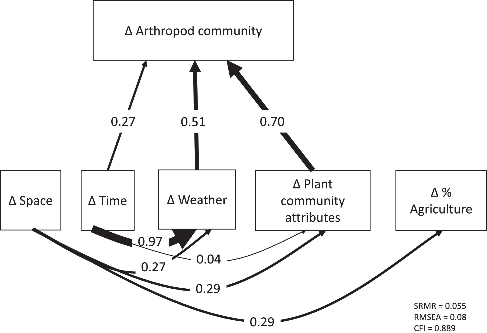
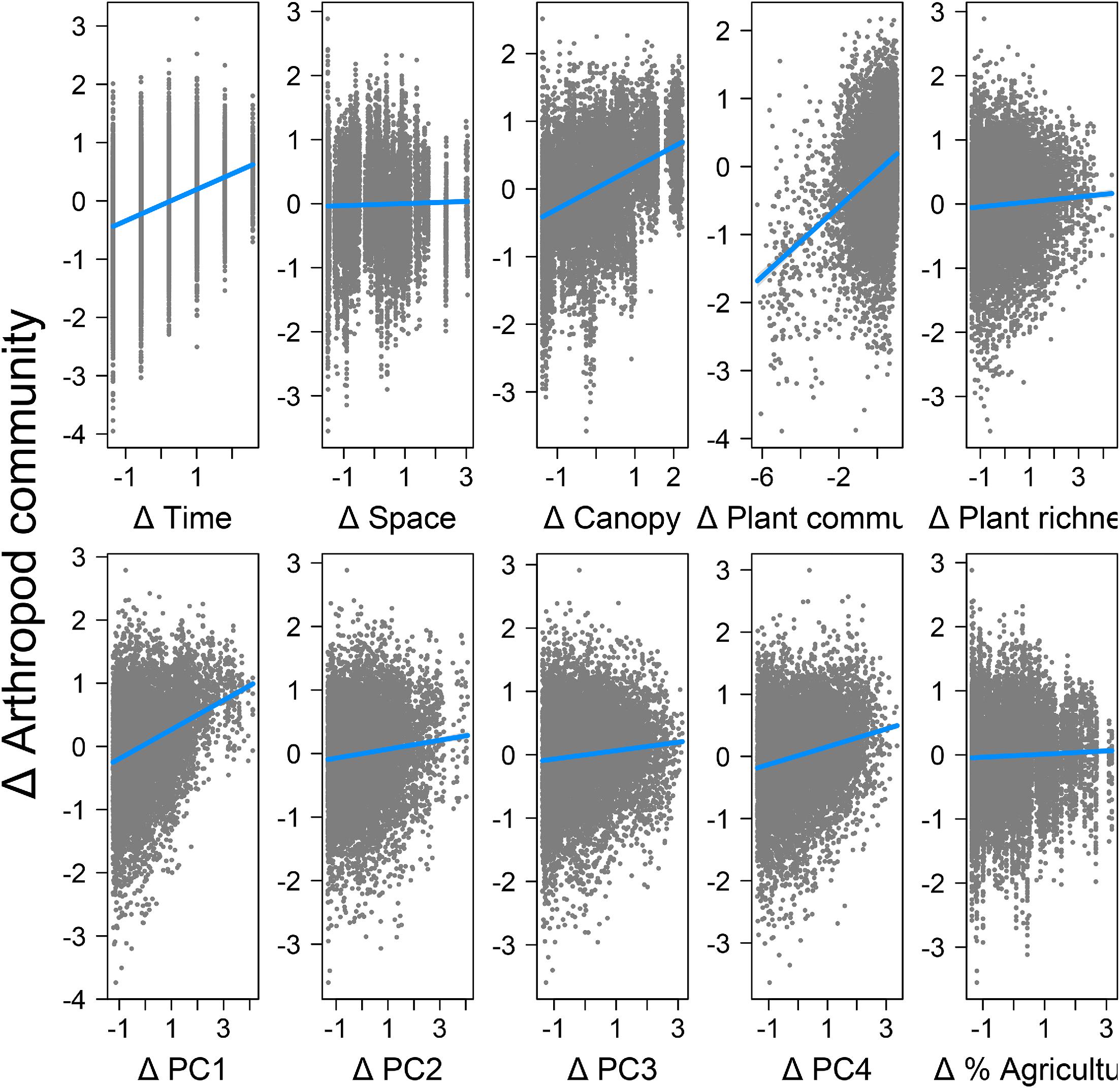
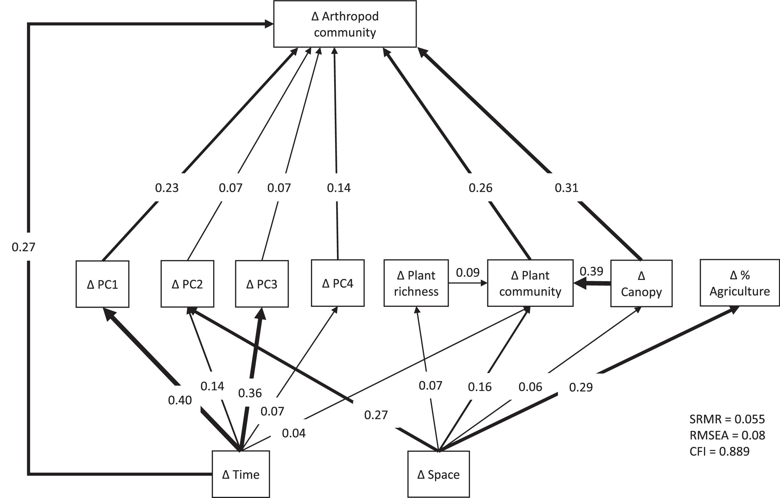
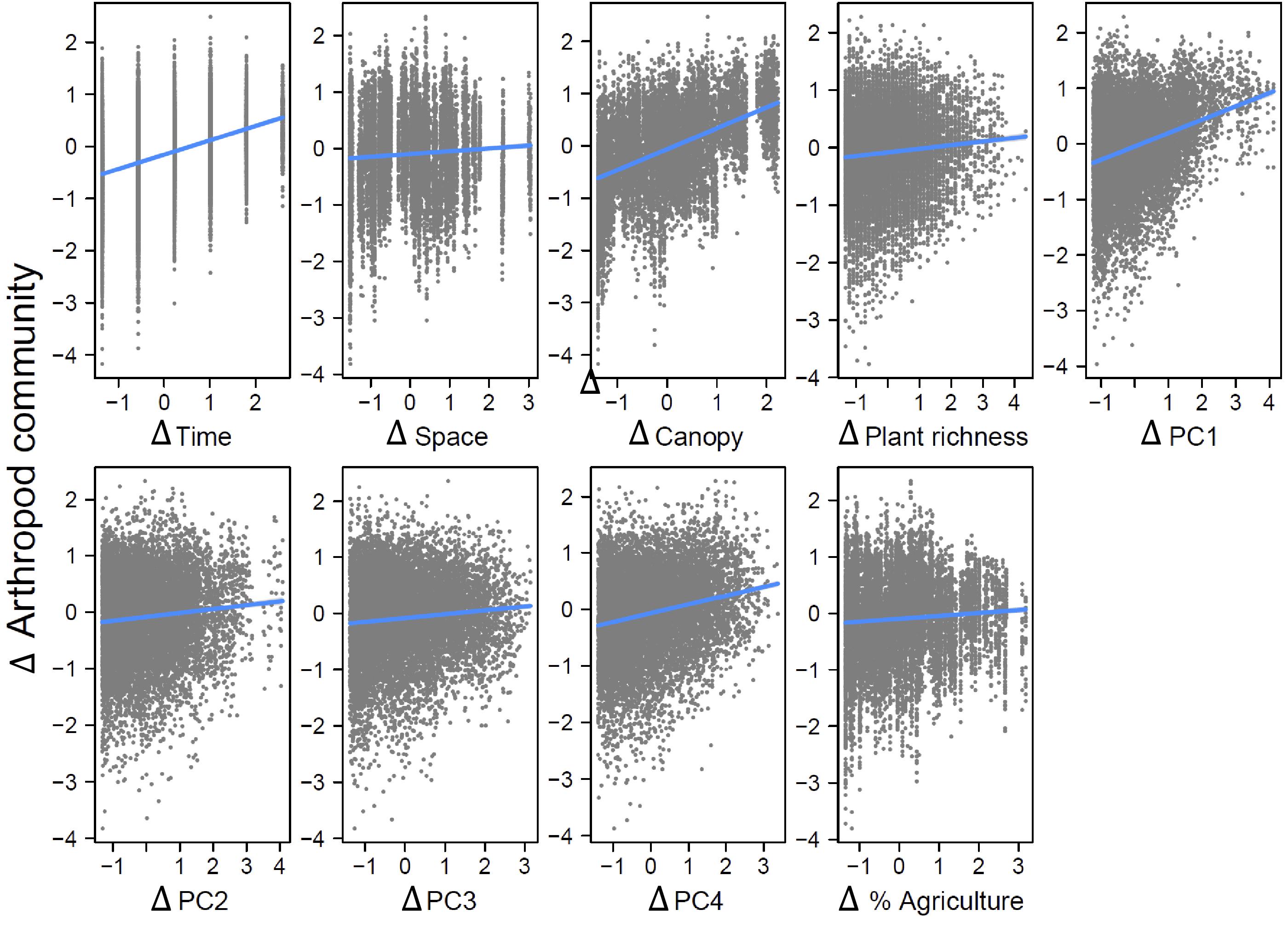
The fit statistics of the path model were as follows: SRMR = 0.055, RMSEA = 0.08, and CFI = 0.889. Arthropod community dissimilarity was significantly related to both environmental distances and temporal distance (SPC = 0.27) (Figs. 57), but there was no significant effect of spatial distance among traps. The total R2 for the effect of all variables on arthropod dissimilarity was 0.49. Spatial and temporal distances were both significantly related to environmental distances (P < 0.05), demonstrating that environmental variables were both spatially and temporally structured. Of the eight environmental variables considered, six had a significant direct effect on arthropod community dissimilarity after Benjamini–Hochberg correction (Figs. 4 and 5). In order of importance, these included a positive effect of changes in canopy openness (SPC = 0.31), a positive effect of plant community dissimilarity (SPC = 0.26), and positive effects of changes in weather variables specified by PC1 (SPC = 0.23), PC4 (SPC = 0.14), PC2 (SPC = 0.07), and PC3 (SPC = 0.07) (Figs. 5 and 6). Loadings of the PCA axes are shown in Table S1 in the Supplemental Information. There was no significant effect of changes in the proportion of agriculture in the landscape nor was there a significant direct effect of plant richness. Plant richness and canopy openness both had indirect effects through compositional dissimilarity among plant communities (SPC with plant community dissimilarity = 0.09 and 0.39, respectively).
Fig. 5.
Fig. 5. Path analysis of standardized variables influencing spatiotemporal Sørensen dissimilarity of arthropod community composition. Only significant paths are shown. Values correspond to standardized path coefficients, and values towards or away from variable groups (e.g., weather) represent the sum of the absolute values of standard path coefficients for each variable within those groups (including direct and indirect effects). Arrow thickness is proportionate to the magnitude of the standardized path coefficients.
Fig. 6.
Fig. 6. Partial regression plots for the effect of all variables in the path analysis on spatiotemporal arthropod Sørensen dissimilarity. PC1 – PCA4 are principal components of the weather variables. All variables are standardized. SRMR, standardized root mean square residual; RMSEA, root mean square error of approximation; and CFI, comparative fit index.
Fig. 7.
Fig. 7. Path analysis of variables influencing spatiotemporal Sørensen dissimilarity of arthropod community composition. PC1 – 4 are principal components of the weather variables. Values correspond to standardized path coefficients. Only significant paths are shown. Arrow thickness is proportionate to the magnitude of the standardized path coefficients.
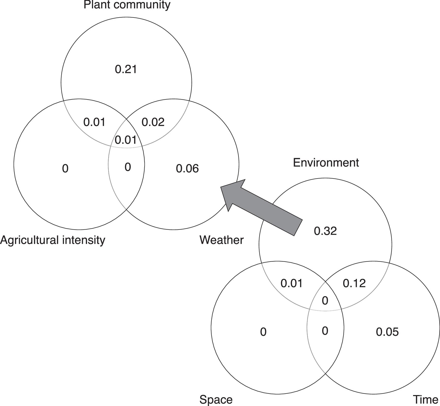
Fig. 8.
Fig. 8. Regression-based variance partitioning results for the effect of distances in environment, space, and time on arthropod Sørensen dissimilarities. Numbers are adjusted R2 values and the results showing the relative effects of plant community attributes, weather, and agricultural extent across the local landscape are conditional on the effects of space and time.
When environmental effects were aggregated into variable groups of weather, plant community attributes, and agricultural extent across the local landscape (Fig. 5), plant community attributes had the strongest effect (Σ|SPC| = 0.70), followed by climate variables (Σ|SPC| = 0.51), with no significant effect of agricultural extent across the local landscape. Plant community attributes and agricultural extent both showed spatial structure (Σ|SPC| = 0.29 for both), while plant community attributes showed weak temporal structure (Σ|SPC| = 0.04), and weather variables showed both temporal and spatial structure (Σ|SPC| = 0.97 and 0.27, respectively).

Variance partitioning

Corroborating the results of the path analysis, variance partitioning (Fig. 7) showed that most of the variation in arthropod community composition could be explained purely by environmental distances (adjusted R= 0.32). Environmental and spatial distances shared a small fraction of variation (adjusted R= 0.01), while spatial distance retained no unique contribution. Environmental and temporal distances shared a larger fraction of variation (adjusted R= 0.12), indicating that temporal variability in environmental conditions across the sampling season played an important role in structuring arthropod communities. Temporal distance retained a unique but small contribution (adjusted R= 0.05). After accounting for the effects of space and time, most of the variation that was explained by environmental distances was due to plant community attributes (adjusted R= 0.21), followed by weather (adjusted R= 0.06), and no unique effect of agricultural extent across the local landscape. These results indicate that much of the effect of local plant communities was trap-specific (independent of spatial and temporal distances), whereas weather variables were largely collinear with temporal distance.

Discussion

Our strongest finding was that spatial variation in arthropod community composition was largely shaped by spatial variation in local floristic composition and weather conditions. These effects dwarfed the impact of spatial variation in agricultural extent across local landscapes, for unknown reasons. We found arthropod communities to be highly variable among localities and across time periods. Plant community attributes best explained this variation. Variability in weather across the sampling season also played an important role. Environmental variables demonstrated both temporal and spatial structure and significant effects of temporal distance on arthropod dissimilarity remained even after accounting for environmental variables, while spatial distance did not retain a significant effect.
It is conceivable that the weak influence of agricultural extent was an artifact of confounded effects among agricultural extent across the local landscape, plant composition, and distance (Fig. 1). Path analysis is designed specifically to accommodate cross-correlation in complex systems to reduce the possibility of such confounding effects (Shipley 2016). We nonetheless repeated the path analysis and variance partitioning after removing the plant composition data. While this alternative model structure resulted in a slightly stronger effect of agricultural extent, it still had much weaker influence on arthropod community dissimilarity than any of the other variables (Figs. S2–S3). Variation in agricultural extent was positively related to distance between our study sites (Fig. S4, P < 0.001, R= 0.083), so it is conceivable that some of the impact of agricultural extent has been incorrectly assigned to distance. Spatial distance was also a weak and statistically insignificant predictor of arthropod beta diversity across our study sites, however, so potential confounding of agricultural extent with distance would not alter our overall conclusion that local variation in plant composition and cover combined with weather variation had the strongest effects on arthropod beta diversity in our study system.
Given that our study landscape supported a mixture of croplands, prairie, wetland, and woodland habitat (Fig. 1), our study sites were no doubt far more heterogeneous than one would normally encounter in regions dominated by industrial farming. Our index of agricultural extent (% cover within a 2 km radius) is rather simplistic, because many different agricultural characteristics contribute to intensification effects on flora and fauna (Beckmann et al. 2019). Resolving this issue will probably require a properly balanced design that is focused directly on more highly detailed comparison between sites with widely differing farming practices.
Canopy openness had a significant direct effect on differences in arthropod community composition, whereas plant richness did not, though both had indirect effects through plant community composition. It is noteworthy that plant richness alone did not have a significant direct effect in our analyses, as many studies have shown this to be an important determinant of arthropod community composition (Borer et al. 2012; Ebeling et al. 2018). Combined with the indirect effect through plant community composition, this means that the identities of plants mattered more than simple measures of richness for the arthropod communities studied here (e.g., Harvey and MacDougall 2015). This could be due to species-specific preferences for food (either directly on plants or other organisms that depend on those plants), nesting, shelter, and mating resources, or because plant community composition also acts as a reliable index of other environmental factors such as light availability or soil type (Schaffers et al. 2008). If the functional and/or nutritional diversity of plant communities is low, it is thus likely that fewer arthropod taxa and functional groups will be represented in these communities (Dolezal et al. 2022).
Taken together, these findings suggest that restoration of multiple habitat types with compositionally distinct plant communities at a local scale is likely to be an effective method for improving arthropod diversity in agroecosystems, provided that the landscape contains enough functionally connected habitat to maintain the species pool (Scheper et al. 2013). Such an approach is exemplified well by Windsor et al. (2021) via their use of network analyses to identify functionally complementary plant mixes that maximize arthropod biodiversity and ecosystem service provisioning in agroecosystems. Beta diversity enhancement through habitat modification is often promoted as one way of mitigating the biodiversity crisis, although it is a crude metric that can be enhanced as readily by addition of invasive species as by restoration of endemic species (Socolor et al. 2016).
Variation in weather conditions, particularly across the growing season, also played an important role in determining arthropod community composition. This could be explained by several mechanisms. The first is that weather has a direct effect on arthropod survival and reproduction. Arthropods are generally constrained to narrow optimum ranges of temperature and humidity and taxa differ widely in their tolerances for climatic conditions, with some species being specialized for early emergence (Høye and Forchhammer 2008). Such differences in the phenology of emergence due to weather conditions results in compositional turnover throughout the season. It could also partially explain why strong differences were observed with forest canopy, as turnover of arthropods between shaded cool forest and warmer and often drier herbaceous plant communities tends to be high (Yekwayo et al. 2017). A related explanation could be resource limitation. Many arthropods depend on specific feeding and nesting/shelter resources, and many of those resources are not available early in the season due to plant phenology in the case of herbivores (foliage) and pollinators (flowers), and the phenology of prey in the case of predators (Høye and Forchhammer 2008).
Much of the variation in arthropod community composition could be explained by environmental variables. The effect of spatial distance on community dissimilarity was not significant after accounting for environmental variation. This finding is especially interesting, given the large extent of our study region and degree of crop monoculture, the fact that many non-crop areas with natural or restored plant cover can be highly spatially isolated (Fig. 1), and that this habitat isolation has been in place for many decades given that this region has been intensely farmed since at least the 1930 s (Riley 2013; McQuarrie 2014). This degree of habitat transformation over the last century might imply acute species turnover by spatial distance but this was not the case.
That being said, single individuals of many flying arthropods such as some species of bee have foraging ranges upwards of 5 km (Greenleaf et al. 2007) and are likely to travel much further in windy conditions (Pasek 1988), resulting in many transient individuals being caught in the traps and high dispersal potential. Indeed, one might expect an arthropod community dominated by highly mobile species in a region that has been repeatedly glaciated in the past. As well, the introduction of dietary and/or eDNA could lead to BIN identifications that are not representative of the immediate trap vicinity (Braukmann et al. 2019). This DNA would likely be relatively diluted and thus less likely to be detected but is an important consideration in the interpretation of results nonetheless.
The effect of time, however, did remain significant after controlling for environmental variation. It seems likely that this is largely due to interspecific differences in the timing of emergence and other life history traits of insects and other arthropods that are linked to seasonal events. No doubt the seasonal cues for such events go well beyond the simple set of weather signals we have analyzed. Periodic seasonal dynamics are clearly evident in other field studies of arthropod abundance and biodiversity (Wolda 1978, 1988; Stinson and Brown 1983; Grøtan et al. 2012; Hatosy et al. 2013; Hallmann et al. 2017), but seasonal effects are often neglected in biodiversity studies.
Attaining a better understanding of the mechanisms that govern arthropod communities in agroecosystems has important management implications. If spatial variation in local plant composition proves to also have a strong influence on variation in the composition of arthropod communities, as our work suggests, then the focus of conservation efforts might be best placed on ensuring that a diverse set of plant communities are well represented across the landscape (Economo 2011).
A significant achievement of our study was to provide a demonstration of how DNA metabarcoding can be used for large-scale terrestrial biomonitoring. During the course of our sampling, 3777 of the BINs sampled (26%) matched the DNA of species previously catalogued in the BOLD database. The fact that so many BINs of unknown species identity were recorded (74% of our sample) in a temperate North American region that has been widely sampled for biological diversity highlights the potential utility of bulk DNA metabarcoding as an exploratory lens to assess the limits of our taxanomic knowledge. Our ability to examine the composition of arthropod communities with such broad taxonomic coverage at this spatiotemporal scale was enhanced by the combined use of metabarcoding and Malaise traps (deWaard et al. 2019; Hausmann et al. 2019). Malaise traps are widely available, easily standardized, passive, and capture an enormous number of arthropods from a variety of taxa that represent many functional groups (Karlsson et al. 2020). Metabarcoding provides a standardized method for species assignment even when a species has not been formally described, allows finer taxonomic resolution, speeds sample processing time, and is very cost-effective (Cristescu 2014; Bush et al. 2020). Using barcoding rather than morphological identification can also increase estimates of species richness and beta diversity by revealing cryptic species (Brehm et al. 2016; D'Souza and Hebert 2018), which allows for a more robust assessment to be made about the factors that drive variation in community composition (Bush et al. 2020). The data generated from collaborative biomonitoring programs using a methodology such as this could create a vast repository of data that can address some of the most critical questions in community ecology facing us today (Derocles et al. 2018; Makiola et al. 2020). In particular, the advent of new techniques in network ecology can allow researchers to achieve a more mechanistic understanding of arthropod declines and their consequences for the rest of the ecosystem (Petsopoulos et al. 2021).
There are a few important caveats to consider in interpreting the results of our study. First, our use of DNA metabarcoding could not capture some important information about these communities. Of particular relevance is the fact that DNA metabarcoding does not necessarily yield accurate measures of abundance (Elbrecht and Leese 2015) and hence our arthropod data was analyzed as presence/absence. As well as this, functional information such as sex, life-stage, and body condition cannot be inferred by DNA metabarcoding (Compson et al. 2020). For example, many species are only pests in one life stage and as such it would be valuable to know what life stage the incidence of the species refers to for the proper timing of pest management procedures throughout a growing season (Crimmins et al. 2020). Recent work in this same system has demonstrated that deep learning from computer vision can be used to provide abundance and biomass estimates from photos of Malaise trap samples (Schneider et al. 2021). Given the large proportion of singletons in our samples, DNA metabarcoding of Malaise trap samples would be an unacceptably crude way to identify candidate species of conservation concern. Future studies that link DNA metabarcoding of Malaise trap samples with such computer-vision based techniques to assess abundance at the species level could conceivably overcome some of these barriers.
PCR amplification is well known as a potential source of bias in metabarcoding studies and covered in detail elsewhere (see Zinger et al. 2019). The primers chosen for this project have been demonstrated to amplify across a wide taxonomic range (most Arthropoda and many other invertebrate phyla), which covers the taxa most often collected by Malaise traps (particularly flying insects). Furthermore, any biases that are present are expected to be evenly distributed across samples and sites, and therefore should not affect the conclusions of this study.
Arthropods collected by Malaise traps must enter the head of the trap before falling down into a clear collection bottle, where they sit for one to several days before servicing and proper preservation in a freezer. This design does not readily collect airborne DNA and preserve airborne DNA well for subsequent detection. With that said, you might expect trace amounts of airborne DNA to enter the samples and possibly be detected through high-throughput sequencing. Much like other sources of environmental DNA (e.g., trace amounts of DNA carried on or inside specimens), the “noise” of airborne DNA is expected to be orders of magnitude lower than the “signal” of the target specimens in the sample; in most cases, this (and other) “noise” will be filtered out during data analysis.
It is also important to note that the placement of the traps (often within 100 of a second habitat type) could have resulted in edge effects, and that the local scale of the plant surveys may not have captured all possible relationships between explanatory variables. In particular, it is certainly plausible that at larger scales one might see stronger links between agricultural practices and arthropod communities. Future studies could address edge effects by a design that isolates habitat effects (e.g., placing all traps within a specific habitat rather than close to edge between habitats) and could address possible interactions between agricultural practices, plant communities, and arthropod communities in more detail by conducting plant surveys at entire-site scales. As well as this, our study sites were from a landscape characterized by a heterogeneous mixture of small farms, forest fragments, small wetlands, and grassland patches and our findings are therefore most representative of highly heterogenous agricultural settings. An important future research direction would be to further tease apart specific effects of different farming management practices on arthropod communities.
Acknowledgements

We thank the numerous technical staff at the Center for Biodiversity Genomics for providing logistic support for the Malaise trap program, arthropod sample processing, and the DNA meta-barcoding pipeline. Andrew Gavloski kindly provided landscape maps of the study area. We offer special thanks to the farmers participating in the ALUS (Alternative Land Use System) program, for providing access to restored habitats on their farms on a regular basis. This manuscript benefited greatly from useful editorial suggestions made by 2 reviewers and the FACETS editorial team. Funding for this work was provided by an operating and knowledge transfer grants from the Food from Thought program supported by the Canada First Research Excellence Fund, an NSERC Discovery Grant to JMF, and an NSERC graduate scholarship to PB.

References

Agriculture and Agri-Food Canada. 2020. Annual Crop Inventory 2019. Availablefrom https://open.canada.ca/data/en/dataset/d90a56e8-de27-4354-b8ee-33e08546b4fc [accessed 31 Jan 2021].
Albrecht M., Kleijn D., Williams N.M., Tschumi M., Blaauw B.R., Bommarco R., et al. 2020. The effectiveness of flower strips and hedgerows on pest control, pollination services and crop yield: a quantitative synthesis. Ecology Letters, 23(10): 1488–1498.
Anderson A., Carnus T., Helden A.J., Sheridan H., Purvis G. 2012. The influence of conservation field margins in intenseively managed grazing land on communities of five arthropod trophic groups. Insect Conservation and Diversity, 6, 201–211.
Beckmann M., Gerstner K., Akin-Fajiye M., Ceaușu S., Kambach S., Kinlock N.L., et al. 2019. Conventional land-use intensification reduces species richness and increases production: a global mea-analysis. Global Change Biology, 25, 1941–1956.
Bell G. 2001. Neutral macroecology. Science, 293, 2413–2418.
Beng K.C., Corlett R.T., Tomlinson K.W. 2018. Seasonal changes in the diversity and composition of the litter fauna in native forests and rubber plantations. Scientific Reports, 8, 10232.
Benjamini Y., Hochberg Y. 1995. Controlling for the false discovery rate: a practical and powerful approach to multiple testing. Journal of the Royal Statistical Society Series B: Statistical Methodology, 57, 289–300.
Bertrand C., Baudry J., Burel F. 2016. Seasonal variation in the effect of landscape structure on ground-dwelling arthropods and biological control potential. Basic and Applied Ecology, 17, 678–687.
Borer E.T., Seabloom E.W., Tilman D. 2012. Plant diversity controls arthropod biomass and temporal stability. Ecology Letters, 15, 1457–1464.
Braukmann T.W.A., Ivanova N.V., Prosser S.W.J., Elbrecht V., Steinke D., Ratnasingham S., et al. 2019. Metabarcoding a diverse arthropod mock community. Molecular Ecology Resources, 19, 711–727.
Brehm G., Hebert P.D.N., Colwell R.K., Adams M., Bodner F., Katrin F., et al. 2016. Turning up the heat on a hotspot: DNA barcodes reveal 80% more species of geometrid moths along an Andean elevational gradient. PLoS ONE, 11, e0150327.
Bush A., Monk W.A., Compson Z.G., Peters D.L., Porter T.M., Shokralla S., et al. 2020. DNA metabarcoding reveals metacommunity dynamics in a threatened boreal wetland wilderness. Proceedings of the National Academy of Sciences, 117, 8539–8545.
Chown S.L., Gaston K.J. 1999. Exploring links between physiology and ecology at macro-scales: the role of respiratory metabolism in insects. Biological Reviews, 74, 87–120.
Compson Z.G., McClenaghan B., Singer G.A.C., Fahner N.A., Hajibabaei M. 2020. Metabarcoding from microbes to mammals: comprehensive bioassessment on a global scale. Frontiers in Ecology and Evolution, 8, 581835.
Crimmins T.M., Gerst K.L., Huerta D.G., Marsh R.L., Posthumus E.E., Rosemartin A.H., et al. 2020. Short-term forecasts of insect phenology inform pest management. Annals of the Entomological Society of America, 113, 139–148.
Cristescu M.E. 2014. From barcoding single individuals to metabarcoding biological communities. Trends in Ecology & Evolution, 29, 566–571.
Crossley M.S., Meier A.R., Baldwin E.M., Berry L.L., Crenshaw L.C., Hartman G.L., et al. 2020. No net insect abundance and diversity declines across US Long Term Ecological Research sites. Nature Ecology & Evolution, 4, 1368–1376.
D'Souza M.L., Hebert P.D.N. 2018. Stable baselines of temporal turnover underlie high beta diversity in tropical arthropod communities. Molecular Ecology, 27, 2447–2460.
Derocles S.A.P., Bohan D.A., Dumbrell A.J., Kitson J.J.N., Massol F., Pauvert C., et al. 2018. Biomonitoring for the 21st century: integrating next-generation sequencing into ecological network analysis. In Advances in Ecological Research. Academic Press Inc., pp. 1–62.
deWaard J.R., Levesque-Beaudin V., deWaard S.L., Ivanova N.V., McKeown J.T.A., Miskie R., et al. 2019. Expedited assessment of terrestrial arthropod diversity by coupling Malaise traps with DNA barcoding. Genome, 62, 85–95.
Dolezal A.J., Esch E.H., MacDougall A.S. 2022. Restored marginal farmland benefits arthropod diversity at multiple scales. Restoration Ecology, 30: e13485.
Ebeling A., Hines J., Hertzog L.R., Lange M., Meyer S.T., Simons N.K., et al. 2018. Plant diversity effects on arthropods and arthropod-dependent ecosystem functions in a biodiversity experiment. Basic and Applied Ecology, 26, 50–63.
Economo E.P. 2011. Biodiversity conservation in metacommunity networks: linking pattern and persistence. The American Naturalist, 177, E167–E180.
Elbrecht V., Leese F. 2015. Can DNA-based ecosystem assessments quantify species abundance? Testing primer bias and biomass-sequence relationships with an innovative metabarcoding protocol. PLoS ONE, 10, 1–16.
Fahrig L., Baudry J., Brotons L., Burel F.G., Crist T.O., Fuller R.J., et al. 2011. Functional landscape heterogeneity and animal biodiversity in agricultural landscapes. Ecology Letters, 14, 101–112.
Fan Y., Chen J., Shirkey G., John R., Wu S.R., Park H., Shao C. 2016. Applications of structural equation modeling (SEM) in ecological studies: an updated review. Ecological Processes, 5.
Fourtune L., Prunier J.G., Paz-Vinas I., Loot G., Veyssière C., Blanchet S. 2018. Inferring causalities in landscape genetics: an extension of wright's causal modeling to distance matrices. The American Naturalist, 191, 491–508.
Gámez-Virués S., Perović D.J., Gossner M.M., Börschig C., Blüthgen N., de Jong H., et al. 2015. Landscape simplification filters species traits and drives biotic homogenization. Nature Communications, 6.
Gossner M.M., Lewinsohn T.M., Kahl T., Grassein F., Boch S., Prati D., et al. 2016. Land-use intensification causes multitrophic homogenization of grassland communities. Nature, 540, 266–269.
Greenleaf S.S., Williams N.M., Winfree R., Kremen C. 2007. Bee foraging ranges and their relationship to body size. Oecologia, 153, 589–596.
Grøtan V., Lande R., Engen S., Sæther B.E., Devries P.J. 2012. Seasonal cycles of species diversity and similarity in a tropical butterfly community. Journal of Animal Ecology, 81, 714–723.
Hallmann C.A., Sorg M., Jongejans E., Siepel H., Hofland N., Schwan H., et al. 2017. More than 75 percent decline over 27 years in total flying insect biomass in protected areas. PLoS ONE, 12, e0185809.
Harvey E., MacDougall A.S. 2015. Spatially heterogeneous perturbations homogenize the regulation of insect herbivores. The American Naturalist, 186, 623–633.
Hatosy S.M., Martiny J.B.H., Sachdeva R., Steele J., Fuhrman J.A., Martiny A.C. 2013. Beta diversity of marine bacteria depends on temporal scale. Ecology, 94, 1898–1904.
Hausmann A., Segerer A.H., Greifenstein T., Knubben J., Morinière J., Bozicevic V., et al. 2019. Toward a standardized quantitative and qualitative insect monitoring scheme. Ecology and Evolution, 10: 4009–4020.
Hebert P.D.N., Penton E.H., Burns J.M., Janzen D.H., Hallwachs W. 2004. Ten species in one: DNA barcoding reveals cryptic species in the neotropical skipper butterfly Astraptes fulgerator. Proceedings of the National Academy of Sciences, 101, 14812–14817.
Hendrickx F., Maelfait J.P., Van Wingerden W., Schweiger O., Speelmans M., Aviron S., et al. 2007. How landscape structure, land-use intensity and habitat diversity affect components of total arthropod diversity in agricultural landscapes. Journal of Applied Ecology, 44, 340–351.
Hesselbarth M.H.K., Sciaini M., With K.A., Wiegand K., Nowosad. J. 2019. Landscapemetrics: an open-source R tool to calculate landscape metrics. Ecography, 42, 1648–1657.
Høye T.T., Forchhammer M.C. 2008. Phenology of high-arctic arthropods: effects of climate on spatial, seasonal, and inter-annual variation. Advances in Ecological Research, 40, 299–324.
Hubbell S.P. 2001. The unified neutral theory of biodiversity and biogeography. Princeton University Press, Princeton, New Jersey, USA.
Jabot F., Laroche F., Massol F., Arthaud F., Crabot J., Dubart M., et al. 2020. Assessing metacommunity processes through signatures in spatiotemporal turnover of community composition. Ecology Letters, 23, 1330–1339.
Karlsson D., Hartop E., Forshage M., Jaschhof M., Ronquist F. 2020. The Swedish malaise trap project: a 15 year retrospective on a countrywide insect inventory. Biodiversity Data Journal, 8, e47255.
Kingsolver J.G. 1989. Weather and the population dynamics of insects: integrating physiological and population ecology. Physiological Zoology, 62, 314–334.
Kremen C., Colwell R.K., Erwin T.L., Murphy D.D., Noss R.F., Sanjayan M.A. 1993. Arthropod assemblages: their use in conservation planning. Conservation Biology, 7, 796–808.
Makiola A., Compson Z.G., Baird D.J., Barnes M.A., Boerlijst S.P., Bouchez A., et al. 2020. Key questions for next-generation biomonitoring. Frontiers in Environmental Science, 7, 197.
McDonald R.P., Ho M.H.R. 2002. Principles and practice in reporting structural equation analyses. Psychological Methods, 7, 64–82.
McQuarrie J. 2014. “Tobacco has blossomed like the rose in the Desert”: technology, trees, and tobacco in the Norfolk Sand Plain, c. 1920-1940. Journal of the Canadian Historical Association, 25, 33–62.
Padgham M., Sumner D. 2020. Geodist: fast, dependency-free geodesic distance calculations. R package version 0.0.4. Available from https://CRAN.R-project.org/package=geodist [accessed 31 Jan 2021].
Pasek J.E. 1988. Influence of wind and windbreaks on local dispersal of insects. Agriculture, Ecosystems & Environment, 22–23, 539–554.
Paterson C., Cottenie K., MacDougall A.S. 2019. Restored native prairie supports abundant and species-rich native bee communities on conventional farms. Restoration Ecology, 27, 1291–1299.
Petsopoulos D., Lunt D.H., Bell J.R., Kitson J.J.N., Collins L., Boonham N., et al. 2021. Using network ecology to understand and mitigate long-term insect declines. Ecological Entomology, 46, 693–698.
Prather R.M., Kaspari M. 2019. Plants regulate grassland arthropod communities through biomass, quality, and habitat heterogeneity. Ecosphere, 10, e02909.
Prosser S.W.J., deWaard J.R., Miller S.E., Hebert P.D.N. 2016. DNA barcodes from century-old type specimens using next-generation sequencing. Molecular Ecology Resources, 16, 487–497.
R Core Team. 2020. R: a language and environment for statistical computing. R Foundation for Statistical Computing, Vienna, Austria. Available from  https://www.R-project.org/ [accessed 31 January 2021].
Ratnasingham S. 2019. mBRAVE: the Multiplex barcode research and visualization environment. Biodiversity Information Science and Standards, 3, e37986.
Ratnasingham S., Hebert P.D.N. 2013. A DNA-based registry for all animal species: the Barcode Index Number (BIN) system. PLoS ONE, 8, e66213.
Riley J.L. 2013. The once and future Great Lakes country: an ecological history (Vol. 2). McGill-Queen's University Press, Montreal, Quebec, Canada.
Rosseel Y. 2012. Lavaan: an R package for structural equation modeling. Journal of Statistical Software, 48.
Sánchez-Bayo F., Wyckhuys K.A.G. 2019. Worldwide decline of the entomofauna: a review of its drivers. Biological Conservation, 232, 8–27.
Schaffers A.P., Raemakers I.P., Sýkora K.V., ter Braak C.J.F. 2008. Arthropod assemblages are best predicted by plant species composition. Ecology, 89, 782–794.
Scheper J., Holzschuh A., Kuussaari M., Potts S.G., Rundlöf M., Smith H.G., et al. 2013. Environmental factors driving the effectiveness of European agri-environmental measures in mitigating pollinator loss—a meta-analysis. Ecology Letters, 16, 912–920.
Schneider S., Taylor G.W., Kremer S.C., Burgess P., McGroarty J., Mitsui K., et al. 2021. Bulk arthropod abundance, biomass, and diversity estimation using deep learning for computer vision. Methods in Ecology and Evolution, 13, 346–357.
Schweiger O., Maelfait J.P., Van Wingerden W., Hendrickx F., Billeter R., Speelmans M., et al. 2005. Quantifying the impact of environmental factors on arthropod communities in agricultural landscapes across organizational levels and spatial scales. Journal of Applied Ecology, 42, 1129–1139.
Seibold S., Gossner M.M., Simons N.K., Blüthgen N., Müller J., Ambarlı D., et al. 2019. Arthropod decline in grasslands and forests is associated with landscape-level drivers. Nature, 574, 671–674.
Shipley B. 2016. Cause and correlation in biology. Cambridge University Press, Cambridge, UK.
Socolor J.B., Gilroy J.J., Kunin W.E., Edwards D.P. 2016. How should beta-diversity inform biodiversity conservation. Trends in Ecology & Evolution, 31:67–80.
Stinson C.S.A, Brown V.K. 1983. Seasonal changes in the architecture of natural plant communities and its relevance to insect herbivores. Oecologia, 56, 67–69.
Stork N.E. 2018. How many species of insects and other terrestrial arthropods are there on earth? Annual Review of Entomology, 63, 31–45.
Sydenham M.A.K., Eldegard K., Totland Ø. 2014. Spatio-temporal variation in species assemblages in field edges: seasonally distinct responses of solitary bees to local habitat characteristics and landscape conditions. Biodiversity and Conservation, 23, 2393–2414.
Tuomisto H., Ruokolainen L., Ruokolainen K. 2012. Modelling niche and neutral dynamics: on the ecological interpretation of variation partitioning results. Ecography, 35, 961–971.
Van Klink R., Bowler D.E., Gongalsky K.B., Swengel A.B., Gentile A., Chase J.M. 2020. Meta-analysis reveals declines in terrestrial but increases in freshwater insect abundances. Science, 368, 417–420.
Vellend M. 2010. Conceptual synthesis in community ecology. The Quarterly Review of Biology, 85, 183–206.
Venables W.N., Ripley B.D. 2002. Modern applied statistics with S. Fourth edition. Springer, New York, USA.
Wagner D.L. 2020. Insect declines in the anthropocene. Annual Review of Entomology, 65, 457–480.
Wagner D.L., Grames E.M., Forister M.L., Berenbaum M.R., Stopak D. 2021. Insect declines in the Anthropocene: death by a thousand cuts. Proceedings of the National Academy of Sciences, 118, e2023989118.
Windsor F.M., Tavella J., Rother D.C., Raimundo R.L.G., Devoto M., Guimaraes P.R., Evans D.M. 2021. Identifying plant mixes for multiple ecosystem service provision in agricultural systems using ecological networks. Journal of Applied Ecology 58: 2770–2782.
Wolda H. 1978. Fluctuations in abundance of tropical insects. The American Naturalist, 112, 1017–1045.
Wolda H. 1988. Insect seasonality: why? Annual Review of Ecology and Systematics, 19, 1–18.
Yekwayo I., Pryke J.S., Roets F., Samways M.J. 2017. Responses of ground living arthropods to landscape contrast and context in a forest-grassland mosaic. Biodiversity and Conservation, 26, 631–651.
Zinger L., Bonin A., Alsos I.G., Bálint M., Bik H., Boyer F., et al. 2019. DNA metabarcoding—need for robust experimental designs to draw sound ecological conclusions. Molecular Ecology, 28: 1857–1862.

Supplementary material

Supplementary Material 1 (DOCX / 436 KB).

Information & Authors

Information

Published In

cover image FACETS
FACETS
Volume 9Number 1January 2024
Pages: 1 - 15
Editor: Josephine Gantois

History

Received: 29 March 2023
Accepted: 1 August 2024
Version of record online: 8 November 2024

Notes

This paper is part of a collection entitled Marginal land restoration, biodiversity conservation, and ecosystem services enhancement in agroecosystem landscapes.

Data Availability Statement

The data and analysis code supporting the paper are archived at https://doi.org/10.5061/dryad.j0zpc86pk. The metabarcoding data supporting the results are archived in the following NCBI public research data repository: https://dataview.ncbi.nlm.nih.gov/object/PRJNA856887?reviewer=n0eubrbgc4tte9h7jiodfalkvq.

Key Words

  1. beta-diversity
  2. DNA metabarcoding
  3. Malaise trap
  4. plants

Sections

Subjects

Plain Language Summary

Preserving Biodiversity: The Role of Natural Vegetation in Countering Insect Decline Near Farmlands

Authors

Affiliations

P. Burgess
Department of Integrative Biology, University of Guelph, Guelph, ON N1G 2W1, Canada
Author Contributions: Conceptualization, Data curation, Formal analysis, Investigation, Methodology, Visualization, Writing – original draft, and Writing – review & editing.
G.S. Betini
Department of Integrative Biology, University of Guelph, Guelph, ON N1G 2W1, Canada
Author Contributions: Conceptualization, Investigation, Methodology, Project administration, Resources, Supervision, and Writing – review & editing.
A. Cholewka
Department of Integrative Biology, University of Guelph, Guelph, ON N1G 2W1, Canada
Author Contributions: Investigation and Writing – review & editing.
J.R. deWaard
Centre for Biodiversity Genomics, University of Guelph, Guelph, ON N1G 2W1, Canada
School of Environmental Sciences, University of Guelph, Guelph, ON N1G 2W1, Canada
Author Contributions: Data curation, Investigation, and Writing – review & editing.
S. deWaard
Centre for Biodiversity Genomics, University of Guelph, Guelph, ON N1G 2W1, Canada
Author Contributions: Data curation, Investigation, and Writing – review & editing.
C. Griswold
Department of Integrative Biology, University of Guelph, Guelph, ON N1G 2W1, Canada
Author Contributions: Formal analysis, Methodology, and Writing – review & editing.
P.D.N. Hebert
Department of Integrative Biology, University of Guelph, Guelph, ON N1G 2W1, Canada
Centre for Biodiversity Genomics, University of Guelph, Guelph, ON N1G 2W1, Canada
Author Contributions: Conceptualization, Data curation, Funding acquisition, Resources, and Writing – review & editing.
A. MacDougall
Department of Integrative Biology, University of Guelph, Guelph, ON N1G 2W1, Canada
Author Contributions: Conceptualization and Writing – review & editing.
K.S. McCann
Department of Integrative Biology, University of Guelph, Guelph, ON N1G 2W1, Canada
Author Contributions: Conceptualization, Funding acquisition, Project administration, and Writing – review & editing.
J. McGroarty
Department of Integrative Biology, University of Guelph, Guelph, ON N1G 2W1, Canada
Author Contributions: Investigation and Writing – review & editing.
E. Miller
Department of Integrative Biology, University of Guelph, Guelph, ON N1G 2W1, Canada
Author Contributions: Investigation and Writing – review & editing.
K. Perez
Centre for Biodiversity Genomics, University of Guelph, Guelph, ON N1G 2W1, Canada
Author Contributions: Data curation, Resources, and Writing – review & editing.
S. Ratnasingham
Department of Integrative Biology, University of Guelph, Guelph, ON N1G 2W1, Canada
Centre for Biodiversity Genomics, University of Guelph, Guelph, ON N1G 2W1, Canada
Author Contributions: Data curation, Software, and Writing – review & editing.
C. Reisiger
Department of Integrative Biology, University of Guelph, Guelph, ON N1G 2W1, Canada
Author Contributions: Investigation and Writing – review & editing.
D. Steinke
Department of Integrative Biology, University of Guelph, Guelph, ON N1G 2W1, Canada
Centre for Biodiversity Genomics, University of Guelph, Guelph, ON N1G 2W1, Canada
Author Contributions: Data curation and Writing – review & editing.
E. Wright
Department of Integrative Biology, University of Guelph, Guelph, ON N1G 2W1, Canada
Author Contributions: Investigation and Writing – review & editing.
E. Zakharov
Department of Integrative Biology, University of Guelph, Guelph, ON N1G 2W1, Canada
Centre for Biodiversity Genomics, University of Guelph, Guelph, ON N1G 2W1, Canada
Author Contributions: Data curation and Writing – review & editing.
Department of Integrative Biology, University of Guelph, Guelph, ON N1G 2W1, Canada
Author Contributions: Conceptualization, Funding acquisition, Methodology, Project administration, Resources, Supervision, Writing – original draft, and Writing – review & editing.

Author Contributions

Conceptualization: PB, GSB, PDNH, AM, KSM, JMF
Data curation: PB, JRd, Sd, PDNH, KP, SR, DS, EZ
Formal analysis: PB, CG
Funding acquisition: PDNH, KSM, JMF
Investigation: PB, GSB, AC, JRd, Sd, JM, EM, CR, EW
Methodology: PB, GSB, CG, JMF
Project administration: GSB, KSM, JMF
Resources: GSB, PDNH, KP, JMF
Software: SR
Supervision: GSB, JMF
Visualization: PB
Writing – original draft: PB, JMF
Writing – review & editing: PB, GSB, AC, JRd, Sd, CG, PDNH, AM, KSM, JM, EM, KP, SR, CR, DS, EW, EZ, JMF

Competing Interests

All the authors declare that they have no competing interests.

Funding Information

NSERC

Metrics & Citations

Metrics

Other Metrics

Citations

Cite As

Export Citations

If you have the appropriate software installed, you can download article citation data to the citation manager of your choice. Simply select your manager software from the list below and click Download.

There are no citations for this item

View Options

View options

PDF

View PDF

Media

Tables

Media

Share Options

Share

Share the article link

Share on social media