Ratchet effects revisited: power effects and systematic bias in natural resource management
Abstract
Regulatory ratchets arise when governance appears to be effective, but actually masks a steady loss of natural capital. This occurs when biases in environmental impact assessment (EIA) systematically underestimate the true impact of large developments, generated by statistical convention fixing α at 0.05 (Type 1 error or false positive rate; i.e., the probability of concluding that a development will have an impact when there is none) while β, the false negative rate (failing to detect a true impact, or Type 2 error), is often fixed at 0.2. This asymmetry (β > α) generates a higher likelihood of mistakenly permitting development than mistakenly preventing it. Beyond statistical bias in EIA, routine environmental regulations are often ineffective due to low compliance, inadequate thresholds, and broad exemptions, which tend to cryptically institutionalize net loss. Measuring bias and inefficiency of environmental regulation is foundational to correcting regulatory ratchets and identifying pathways towards no net loss. Like net loss from major developments, cumulative net loss from inadequate routine environmental protections also needs to be estimated and offset by active habitat restoration; this should be delivered as a core program of resource management agencies, with the goal of fully integrating the mitigation hierarchy into routine natural resource governance.
Introduction
Earth is undergoing a steady decline of biodiversity, habitat, and natural resources as humanity transforms natural capital into consumer products, urban and agricultural land, and industrial and domestic infrastructure (Postel et al. 1996; Watson et al. 2018; Richardson et al. 2023). Most developed nations have implemented some form of environmental regulation to minimize ecosystem degradation and associated loss of natural capital (defined broadly here as the abundance of listed and nonlisted species, habitats, and their associated ecological functions; Guerry et al. 2015). These protections are often in the form of environmental impact assessments (EIA) for screening the effects of large development projects, and general environmental regulations (e.g., water quality and riparian protection standards) intended to protect natural capital from the cumulative impacts of routine smaller-scale development. In addition to domestic environmental legislation, many nations have also adopted post-2020 Global Biodiversity Framework targets (e.g., 30% protected area and 30% restoration of degraded ecosystems by 2030) to address ongoing declines in biodiversity, natural habitat, and ecosystem services (Díaz et al. 2020; Xu et al. 2021; Convention on Biological Diversity 2022). In principle, this establishes both a floor on the trajectory of decline of natural capital (30% minimum) as well as a threshold target for recovery (60% total, depending on the spatial overlap between protection and restoration).
Protected areas are essential for conserving biodiversity; however, ensuring no net loss (NNL; Maron et al. 2018) of natural capital outside their boundaries is equally critical to maintaining biodiversity and ecosystem function in developed landscapes (Cox and Underwood 2011; Cowie et al. 2018; Ramírez-Delgado et al. 2022). Decisions to develop or conserve natural capital are based on trade-offs among values related to human well-being (e.g., economic outcomes, ecosystem services) and conservation goals (Dearing et al. 2014; Gillingham et al. 2016). Although trade-offs are ultimately value-based and subjective, science provides an objective framework for collecting and evaluating the biophysical data underlying trade-off decisions. An objective science process is foundational to the accurate prediction of environmental response to human activities, and requires a framework without structural bias (i.e., one that minimizes systematically over- or under-estimating the true ecological impacts of development).
The decline of natural capital is often exacerbated by ratchet effects (Birkeland 2004; Perkin et al. 2015), which are here broadly defined as policy or process that inadvertently facilitates depletion of natural capital (and often obstructs its’ recovery). Ratchet effects exert constant downward pressure and in severe cases may induce feedback loops that amplify pressure over time. A classic example of an economic ratchet is over-investment in fishing fleets during cyclic peaks in stock abundance, followed by overfishing in subsequent periods of low stock productivity (Caddy and Gulland 1983; Ludwig et al. 1993); economic hardship then results in further pressure to exploit dwindling stocks. Regulatory ratchets arise when environmental protection is ineffective or has a significant failure rate (e.g., Quigley and Harper 2006), effectively normalizing environmental degradation despite the appearance of protection, thereby contributing to a trajectory of decline (Quigley and Harper 2006). Although many hidden processes in economic and governance systems contribute to downward pressures on natural capital, science is generally assumed to play a neutral role. However, traditional applications of science to environmental regulation and impact assessment share some of the attributes of a ratchet, and may be inadvertently contributing to the rapid loss of natural capital. Although this issue has been described elsewhere (e.g., Peterman 1990; Mapstone 1995; Kriebel et al. 2001) it remains poorly reported, and implications for managing cumulative effects and global land degradation are under-appreciated in the science community. The objective of this paper is to consider how application of a traditional hypothesis testing framework to EIA and regulation may contribute to a ratchet effect generating downward pressure on natural capital. Although there are many potential statistical and social sources of bias in EIA (e.g., intrusion of subjectivity and conflict of interest: Murray et al. 2018; Singh et al. 2019; impact monitoring duration that is too short to detect lagged effects: Singh et al. 2019; White 2019; political interference: Bragagnolo et al. 2017; Enríquez-de-Salamanca 2018; Bond et al. 2020), the focus here is on (i) ratchet effects associated with transposing conventional treatment of Type 1 and Type 2 errors to environmental assessment and regulation; (ii) ratchet effects associated with routine environmental regulation outside of EIA; and (iii) the governance structures required to correct these biases, as described below.
Cryptic biases associated with the statistical treatment of uncertainty
Conventional research usually involves testing the null hypothesis of no difference between treatment and control versus the alternative hypothesis of a significant treatment effect. This entails two sources of error: Type 1 error (α), which represents the probability of a false positive (i.e., falsely concluding that the treatment differs from the control when the observation is simply an outlier; Fig. 1A); and Type 2 error (β) which is the probability of a false negative, i.e., falsely concluding that treatment and control are identical—no impact—when in fact there is a difference, but the analysis lacks sensitivity to detect the effect (Fig. 1; Biau et al. 2010). 1-β represents statistical power, i.e., the power of an experimental or monitoring design to detect a treatment effect (Fig. 1A; Peterman 1990).
Fig. 1.
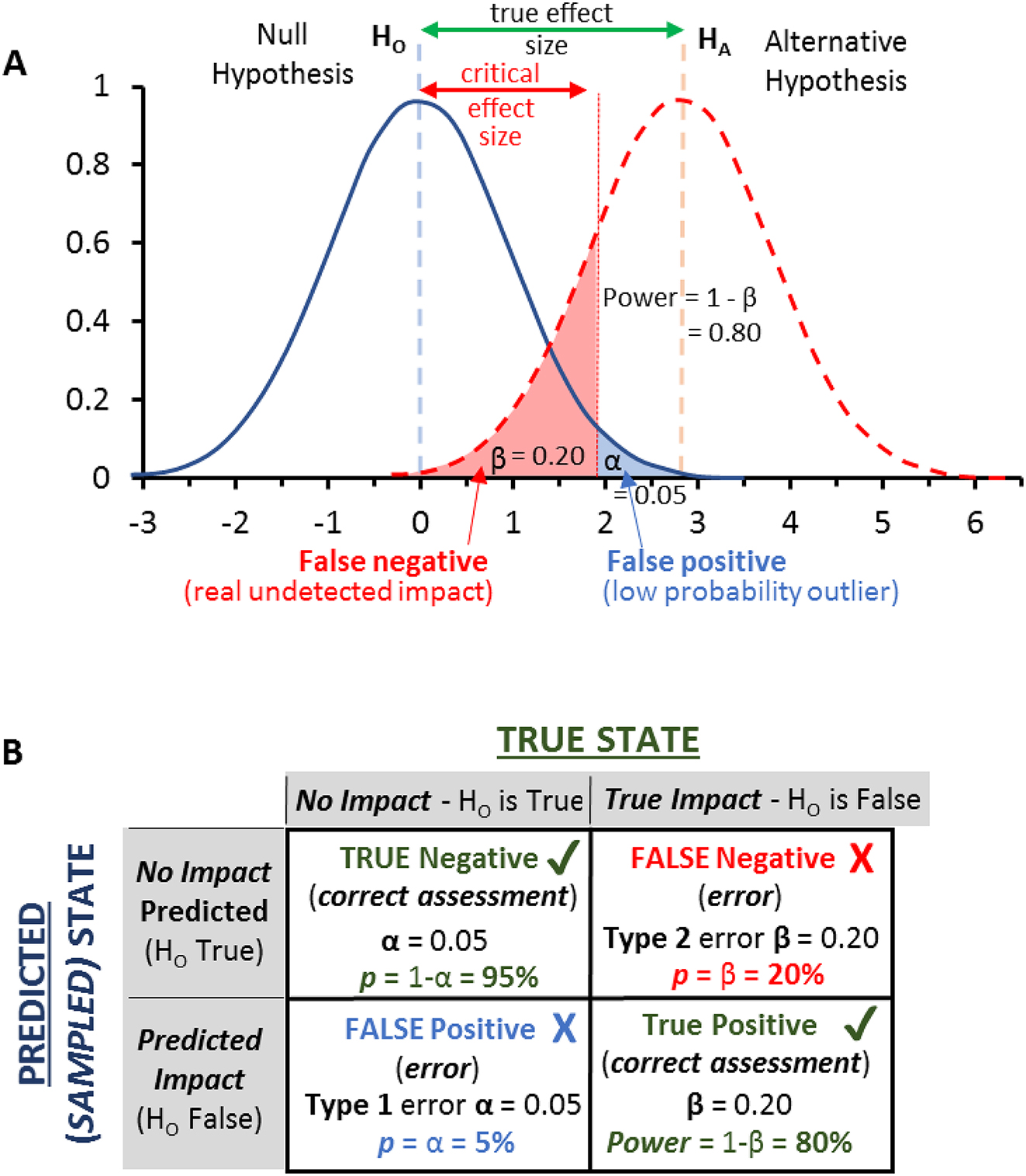
In traditional research, the primary goal is to detect or demonstrate a treatment effect, and a significant effect is generally the trigger for scientific progress; failure to detect a treatment effect may stimulate more research with increased replication and better error control, but absence of a treatment effect usually indicates a dead end for any particular research hypothesis (Mapstone 1995). By convention, the Type 1 error α is generally set at α = 0.05 (i.e., a 5% probability of falsely concluding that there is a treatment effect). There is also a trade-off between Type 1 and Type 2 errors (Fig. 1A); a decrease in α (e.g., from 0.05 to 0.01) right-shifts the significance threshold and decreases the likelihood of a Type 1 error, but increases the likelihood of a Type 2 error.
While scientists try to design experiments with adequate power to detect treatment effects, the likelihood of a Type 2 error is usually not fixed, but varies depending on statistical design; however, by convention the default target power is often set at an 80% probability of detecting a treatment effect (β = 0.2) implying that the true effect will go undetected 20% of the time (Fig. 1B; Cohen 1988; Biau et al. 2010). This asymmetry (5% error rate for false positives, 20% for false negatives) reflects the premium placed on avoiding a mistaken conclusion that a treatment effect exists when it does not (i.e., a false positive), since this could cause significant investment in a nonsensical research trajectory and potentially lead to harm if false results are applied, for instance in a medical setting (Shrader-Freshette and McCoy 1992). On the other hand, failing to detect a true treatment effect (false negative or Type 2 error), while a potential lost opportunity cost to basic science, is less likely to lead to active harm. In effect, the implicit trade-off between Type 1 (α = 0.05) and Type 2 error (β = 0.2) in traditional science places a premium on minimizing false positives (falsely concluding that treatment effects exist) over false negatives (falsely concluding that treatment effects are absent), and is precautionary towards confidence in inferring true treatment effects over their absence (Peterman 1990; Shrader-Freshette and McCoy 1992; Mapstone 1995; Kriebel et al. 2001).
In contrast, the causality of action based on hypothesis testing is reversed in the field of EIA; the absence of a treatment effect (no predicted environmental impact) is what triggers action, in the form of economic development. A false positive (Type 1 error indicating that development will cause impact when this is false) typically has a fixed probability α = 0.05, effectively making the assessment process precautionary towards development interests (low likelihood of lost development opportunities). In contrast, power to detect an impact (false negative) is generally lower, and varies across assessments depending on replication, the threshold effect size for detection of impact, and other aspects of monitoring and experimental design (Andrew and Mapstone 1988; Peterman 1990; Mapstone 1995), but the default target power is often 80% (Cohen 1988). In this sense, the reverse causality of action between traditional research hypotheses (insignificant treatment effect results in no action) and development under EIA (insignificant treatment effect triggers development) makes low power differentially protective of development interests (Mapstone 1995). In other words, a fixed α = 0.05 and a variable but generally higher β means that the likelihood of mistakenly authorizing a significant environmental impact is usually higher than the likelihood of mistakenly preventing development.
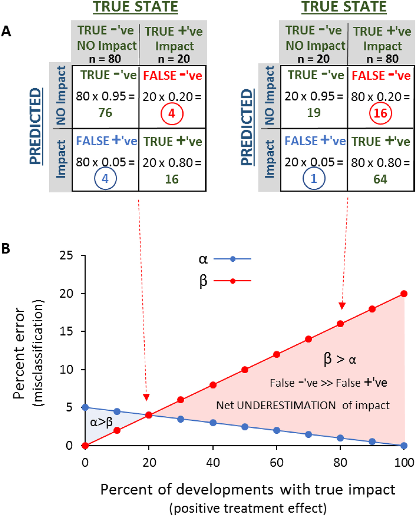
This asymmetry in predicted risk is very sensitive to the true frequency of development impact (Biau et al. 2010), as illustrated in Fig. 2. For example, if the true frequency of impact is 80% for a hypothetical population of 100 proposed developments, then 80 out of 100 will experience impacts exceeding a specified critical effect size, and 20 will remain unaffected (Fig. 2A, right table). If α = 0.05, then of the 20 unimpacted sites, 20 × 0.05 = 1 will be misclassified as impacted (false positive, hypothetically causing lost development opportunities). If β = 0.2, then 80 × 0.2 = 16 of the impacted sites will be misclassified as unimpacted when in fact they would be impacted by development (false negatives, hypothetically leading to environmental harm). In this case of an 80% true frequency of impact vulnerability, false negatives (16%) greatly exceed false positives (1%), meaning that the assessment process is far more precautionary to development interests than the environment (15% net underestimation of impacted sites; Fig. 2B; red shaded area in Fig. 1A). In contrast, precaution towards environmental impacts only emerges at low frequency rates of true impact (Fig. 2). If the true frequency of realized impact from a hypothetical development is 20% (see calculations in Fig. 2A left table), then the frequency of false negatives is equal to the frequency of false positives (Fig. 1D), and the process is equally precautionary to both economic and environmental interests (4% misclassification rate for both; Fig. 2). At higher frequencies of true impact there is a clear bias in favour of underestimating development effects, driven by the low power to detect them (default 80% power, β = 0.2). Mapstone (1995) discusses the balance between Type 1 and Type 2 error rates, how it affects development versus environmental protection interests, and describes a process for covarying α and β thresholds to achieve equal weighting of uncertainty (α = β) and therefore economic and environmental consequences. While this more nuanced approach has merit and experienced EIA practitioners may use it, traditional assessment with α fixed at 0.05 remains the general default.
Fig. 2.
This example presents a simplified picture of the overall environmental assessment process, which often involves additional iterative steps to minimize risk beyond what is considered here; nevertheless, it captures a very real bias in the underlying statistical logic. In principle, the potential for bias will apply to assessment of impacts during post-assessment monitoring, as well as the initial screening and assessment of whether a development should proceed (assuming the decision involves inferential statistics).
EIA is a complex process generally applied to very large developments, with impacts that are often unique to each project. In contrast, the many routine impacts of most small developments are regulated with general environmental standards (e.g., fixed water quality thresholds or riparian buffer widths). Fixed regulatory standards have the advantage of eliminating the need to assess uncertainty around impacts on a site-by-site basis; however, the degree to which standards meet or fall short of a reference (unimpacted) condition is effectively built into the regulation itself, and many regulatory approaches ensure only partial protection of natural capital or ecosystem function (Lemieux et al. 2019; Zu Ermgassen et al. 2019). For example, streamside riparian buffers play a critical role in protecting production of stream salmonids by ensuring shade, recruitment of large wood essential to pool formation, and maintenance of channel complexity (Richardson et al. 2010; Rosenfeld et al. 2024). Riparian buffer widths may be wide enough to ensure close to 100% of reference wood input levels on anadromous fish-bearing streams on public land in some jurisdictions (e.g., Alaska; Murphy 1995), but elsewhere narrower buffers on small forested streams may retain only 80% of reference levels of large wood inputs (e.g., Johnston et al. 2007), indicating a fractional loss of natural capital, i.e., the regulation itself may have an embedded and often cryptic trade-off between economic and environmental values. Complete absence of riparian protection on agricultural streams (e.g., British Columbia Ministry of Forests, Lands, and NRO 2019) represents a more extreme but less cryptic failure to protect natural capital by explicit exemption. In addition, beyond these design limitations most regulations also have significant failure rates associated with incomplete compliance, enforcement, or mitigation (Zu Ermgassen et al. 2019; Third et al. 2021). For example, a decade after riparian regulations were brought into force in 2005 in the Province of British Columbia, Canada, 17% of local governments were found to be noncompliant (Office of the Ombudsperson of British Columbia 2022). Consequently, there will almost always be residual impacts of development even with well-intended regulations (i.e., the product of embedded limitations and lack of compliance), again contributing to a potential ratchet effect.
Random errors in parameter estimates are typically equally distributed around the mean if an estimation procedure is without bias, leading to a reasonable expectation that on average management decisions should also be without bias (overestimations equal underestimations). However, in the field of environmental regulation positive and negative errors do not necessarily balance. Type 2 errors (false negatives, where potentially harmful developments are greenlighted) lead to loss of natural capital. In contrast, Type 1 errors (false positives where environmentally benign developments do not proceed) do not result in an equivalent increase in natural capital; at best they result in NNL. Therefore the combined cumulative impacts of neutral Type 1 errors and negative-effect Type 2 errors will always be a directional net loss of natural capital, again supporting a ratchet effect. This circumstance applies equally to EIA (large developments) and application of routine regulatory standards. The potential for ratchet effects will often be compounded by relatively large detection thresholds associated with low statistical power (Fig. 1). Biological data are notoriously variable, and effect size detection thresholds on the order of 50% of the mean or greater are not uncommon (e.g., Steidl et al. 1997), and 25% is often used as a detection threshold in environmental monitoring (Munkittrick et al. 2009); the implication being that substantial impacts may go undetected, masking potentially significant cumulative effects when aggregated across landscapes.
Offsetting (e.g., restoration to compensate for habitat loss) is widely promoted as a pathway to remedy the negative environmental impacts of development, with variable success (Quigley and Harper 2006; Rey Benayas et al. 2009; Quétier et al. 2014; Guillet and Semal 2018). If conventional statistics are used to calculate the magnitude of impact that needs to be offset, then the arguments above indicate that most offsetting requirements (i.e., multipliers) will be underestimated. The concept of offsetting is also typically applied to mitigate the impacts of large developments associated with detailed EIAs. However, the logic above makes a strong case that some form of off-setting also needs to accompany routine environmental regulations (e.g., riparian protection legislation), where incomplete compliance generates cumulative impacts that require mitigation to avoid net loss, despite apparently protective regulation.
While concerns are well established that statistical convention setting α ≪ β biases detection of treatment effects, some recent studies have highlighted the opposite effect. Low-probability events that document significant impacts on biodiversity may represent Type 1 errors (false positives), with their significance amplified through selective publication (Lemoine et al. 2016; Yang et al. 2022). However, this selection bias is unlikely to be a concern in routine EIA, which are rarely published in the primary literature and therefore not subject to a filter that amplifies significant results.
Statistical interpretation of the precautionary principle
The precautionary principle (often stated as “a lack of full scientific understanding shall not be used as a reason for postponing cost-effective measures to prevent environmental degradation”; Rio Declaration, UNECP 1992; Cooney 2004) is frequently promoted as a conservative approach to deal with uncertainty in natural resource management (e.g., Raffensberger and Barrett 2001; Sachs 2011). However, it is often strongly opposed by stakeholders who see it as a mechanism to obstruct development (Sunstein 2003; Turner and Hartzell 2004), not the least because it’s meaning and interpretation is poorly defined (O'Riordan and Jordan 1995; Foster et al. 2000). Consequently, it sees limited practical application, despite being recognized as a guiding principle in policy and legislation (Foster et al. 2000).
The preceding discussion on Type 2 errors provides the foundation for an objective interpretation of the precautionary principle, where the goal is not to wield uncertainty as a blanket rationale for obstructing development, but to explicitly correct the inherent biases described above. Practical implementation of this precautionary approach could be challenging, but would be based on explicit recognition of the anticipated rate of false negatives (or other quantifiable biases; e.g., Thompson et al. 2000) and the need to eliminate them. For example, if asymmetry in Type 1 and Type 2 errors means that 15 out of 100 developments are false negatives (e.g., Fig. 2), then in principle 15% of projects could cause environmental harm and should not proceed or would require additional offsetting. In this example, a precautionary approach at the population or landscape level of multiple development projects could support a goal of identifying the 15% of highest risk projects pre-approval based on information that may have been excluded from initial quantitative screening or pre-impact monitoring, or using alternative weight-of-evidence approaches (Plowright et al. 2008; Downing et al. 2010). At the project assessment level, it could mean better balancing Type 1 and Type 2 error (i.e., equal allocation of risk to the environment vs. development interests), either through formal statistics (adjusting α = β; Mapstone 1995) or by qualitative assessment of acceptable threshold effect sizes. However, even when α and β are equal, any error will still lead to net loss and require some form of additional offset, albeit at a reduced rate. Empirical estimation of EIA error rates (i.e., impact misclassification) would be useful to establish the true frequency and magnitude of error, and could in principle be derived from retrospective comparison of predicted versus realized impacts extracted from pre- and post-impact reporting for a population of project assessments.
Ultimately, correcting the biases identified above requires some degree of process and institutional change. A shortlist of priority actions to minimize the impacts of regulatory and institutional rachets in environmental governance follows.
Fig. 3.
Key recommendations
i.
Management agencies and policy makers need to avoid complacency around the assumed effectiveness of environmental regulations. Routine effectiveness assessment of environmental regulations needs to be institutionalized to objectively evaluate the degree to which regulations are achieving NNL (e.g., Harper and Quigley 2005; Quigley, et al. 2006).
ii.
Accurate accounting of natural capital and projected impacts of development (Guerry et al. 2015; Bull et al. 2018) is central to efforts to achieve NNL or land degradation neutrality (LDN, which is NNL in the amount and quality of resources necessary to support ecosystem functions and service at landscape scale; Cowie et al. 2018). The cumulative effects of real impacts that are below detection thresholds (e.g., Fig. 1) can be significant at a landscape scale, and need to be taken into account to properly inform restoration and off-setting objectives. Simple but credible methods need to be developed to estimate the frequency and magnitude of these below-threshold-of-detection impacts (e.g., based on assumed, measured, or modelled frequency distributions of impact magnitude), to avoid underestimating both cumulative effects and mitigation needs.
iii.
The concept of offsetting within a mitigation hierarchy (first priority to avoiding impacts, followed by minimizing impacts when avoidance is not possible, with restoration/offsetting as a last resort; Arlidge et al. 2018) is now widely accepted with the goal of achieving NNL for development projects that trigger EIA. However, a need to implement restoration/offsetting to deal with shortcomings in application of routine management regulations (e.g., riparian protection or water quality laws not necessarily associated with new development projects) also needs to be recognized. More specifically, agencies responsible for environmental protection need to develop complementary landscape-scale habitat restoration programs to offset the cumulative impacts associated with the failure of routine environmental regulations to achieve NNL objectives. This expansion of responsibilities would also provide an unparalleled opportunity to integrate First Nations governance into natural resource management, stewardship, and restoration, in support of both reconciliation and more effective restoration (Artelle et al. 2019; Lamb et al. 2022; Grenz and Armstrong 2023).
iv.
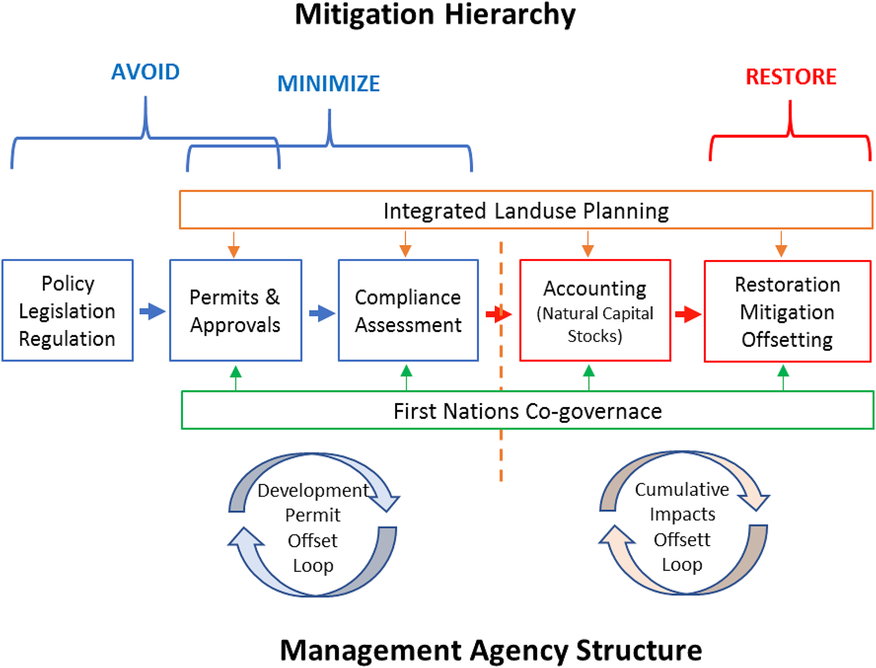
There is a need to better integrate the mitigation hierarchy (Arlidge et al. 2018) into the administrative structure of natural resource management agencies to achieve NNL and LDN (Díaz et al. 2019; Ray et al. 2021). Many natural resource management agencies focus on the necessary steps of developing environmental policy, regulations, and to a lesser degree regulatory compliance (Fig. 3). However, these represent only the first and second steps in the mitigation hierarchy. Divisions within agencies that actively focus on restoration and offsetting (both on-the-ground delivery and higher-level coordination) are needed to close the loop on the full process leading to LDN (Fig. 3).
However, managers and policy makers also need to maintain realism around the ability of restoration and offsetting to compensate for regulatory failures (Palmer and Filoso 2009; Rey Benayas et al. 2009; Maron et al. 2012); limits to the effectiveness of restoration and the availability of suitable offset sites inevitably limits capacity to compensate for lost habitat (Quétier et al. 2014; Schulp et al. 2016; Zu Ermgassen et al. 2019). Offsetting must be treated as a tool to supplement largely effective regulatory regimes, rather than as a solution to poorly functioning and ineffective environmental regulation. Any perception that unlimited development can be effectively mitigated through restoration and offsetting needs to be confronted as a delusion (Maron et al. 2012; Moore and Moore 2013; Spash 2015).
v.
Achieving NNL/LDN at a regional of landscape scale requires integration of NNL objectives with landuse planning and development authorizations over multidecadal time projections (Kiesecker et al. 2010; Titeux et al. 2016). Identifying optimal development scenarios (Cook et al. 2014) will then constrain the scale and location of proposed authorizations that are compatible with long-term goals. Local and regional offices of natural resource management agencies need to align the trajectory of short-term landuse planning, permitting, and approval processes with optimal long-term development scenarios in support of NNL or other defined targets (Kiesecker et al. 2010; Cowie et al. 2018).
Conclusion
Advances in technology have decoupled human populations from classic density-dependence, resulting in accelerating depletion of natural capital (i.e., ratchet effects). The challenge for natural resource governance is to develop regulatory frameworks and management interventions as substitutes to classic density-dependent feedback mechanisms, with the goal of achieving NNL in human-modified landscapes. Regulatory ratchets emerge when regulations appear to be effective, but in fact mask a net loss of natural capital due to biases in EIA, liberal regulatory impact thresholds (Chapron et al. 2017), or low compliance with routine environmental regulations. The mitigation hierarchy of avoid, reduce, and restore (Arlidge et al. 2018; Cowie et al. 2018; Zu Ermgassen et al. 2019) is recognized as fundamental to achieving land degradation neutrality, but requires accurate evaluation of the magnitude of impacts on natural capital. This requires a clearer understanding of the systemic biases in current environmental assessment and environmental regulation that are ratchetting loss of natural capital faster than expected, and how to correct for these biases. Natural resource management decisions will remain contentious because of conflicts between the fundamental values of conservation versus development. However, in an era of increasing disinformation (Shu et al. 2020), science plays a critical role in objectively assessing the consequences of development decisions, and an accurate accounting of bias and uncertainty is key to realistic projections of future state.
The statistical asymmetry between committing a Type 1 error (falsely inferring an impact, α = 0.05) versus a Type 2 error (β = 0.2) is well understood by statisticians and those well-versed in statistical analysis and design, but the implications for natural resource management (i.e., greater precaution towards development interests over the environment) are less widely appreciated. While advice exists to mitigate this bias (e.g., equalize α and β; Mapstone 1995), it is unclear how widely this is applied in routine EIA. Of equal concern are impacts that fall below minimum detectable effect size thresholds (e.g., 25% of the mean; Munkittrick et al. 2009), but have the potential to accumulate across multiple projects and landscapes. Understanding the scope and magnitude of these collective biases is key to improving the practice of environmental regulation, and to accounting for their contribution to declines in stocks of natural capital (Guerry et al. 2015).
Of equal importance to accurate accounting of natural capital is a commitment and capacity to mitigate routine cumulative development impacts that are not covered by large project assessments (Favaro and Olszynski 2017; Third et al. 2021). However, one of the risks of adopting the restoration/offsetting paradigm is it’s vulnerability to devolution into performative greenwashing that facilitates development and undermines the urgency of real habitat protections (Moore and Moore 2013; Spash 2015; Le Billon 2021). This concern is validated by widespread implementation failures of NNL policies (zu Ermgassen et al. 2019; Aminian-Biquet et al. 2024). For instance, studies as early as 2006 demonstrated aggregate net loss of aquatic habitat in Canada (Harper and Quigley 2005; Quigley et al. 2006), despite introduction of a credible NNL policy two decades earlier (DFO 1986); this situation persists today (Favaro and Olszynski 2017; Third et al. 2021), indicating deep institutional constraints on effective implementation of the mitigation hierarchy. Like EIA, most offsetting and restoration in support of NNL is carried out by private contractors who’s activities are usually monitored by the proponent (i.e., developer), arguably creating a conflict of interest (Singh et al. 2019) and potentially facilitating industry capture of the regulatory process (Dal Bo 2006; MacLean 2016). This poorly regulated service delivery model, compounded by a lack of landscape-scale coordination and natural capital accounting, is likely a major contributing factor to the administrative and implementation failures of NNL policies. Creating permanent capacity for public institutions to directly engage in and coordinate restoration/offsetting around cumulative impacts (secondary offset loop in Fig. 3) in partnership with First Nations, NGOs, industry, and other stakeholders, would go a long way towards addressing the mismatch between NNL policy and realized outcomes. Several studies make the case that greater indigenous involvement in resource governance would increase effectiveness and efficiency because (i) much of the remaining high quality habitat with minimal development impact is under current or historic indigenous governance, necessitating their participation (Artelle et al. 2019); (ii) indigenous traditions, technologies, and values are inherently more sustainable than extractive western management practices (Atlas et al. 2021); and (iii) local management tends to be more efficient and context-appropriate (Stoa 2014).
The disaggregated nature of governance structures and land use planning decisions is also a significant obstacle to maintaining natural capital (Hodgson et al. 2019). Achieving NNL (or any landscape-scale goal) requires collaborative integrated planning to coordinate activities and value trade-offs across resource sectors, agencies, and jurisdictions (municipal, provincial, federal; Gillingham et al. 2016; Chan et al. 2020; Ray et al. 2021; Cormier et al. 2022). While the need for co-ordinated land use planning is widely recognized (e.g., Council of Canadian Academies 2019; Hodgson et al. 2022), conflicting interests, policies, and power asymmetries between agencies responsible for conservation vs. resource extraction can complicate integrated management (Collard et al. 2020; Ray et al. 2021). Conflicts can arise, for instance, when an agency responsible for managing aquatic habitat (e.g., the federal government in Canada) adopts a NNL policy, but agencies responsible for managing upslope terrestrial habitat (e.g., provincial governments) do not (Ray et al. 2021); this can make achieving NNL of aquatic habitat extremely difficult, given the pervasive influence of terrestrial land use on aquatic habitat quality (Allan 2004; Feld et al. 2018). While challenging, these conflicts can be negotiated through broader policy and management agreements within or across jurisdictions. Examples include the EU Biodiversity Strategy, Marine Strategy, and Water Framework directives that set out shared international goals for EU member states (Acreman and Ferguson 2010; Lyons et al. 2010; Schulp et al. 2016; note, however, that these higher-level international directives can have significant failings, e.g., Flávio et al. 2017; Voulvoulis et al. 2017; Cavallo et al. 2019); the bilateral United States-Canada International Joint Commission, which was instrumental in managing transboundary pollution and eutrophication in the Laurentian Great Lakes (Duda 1994; Clamen and Macfarlane 2015); and regional agreements to jointly manage natural capital, such as collaborative watershed planning involving provincial governments and First Nations (Nicola Watershed Governance Partnership 2018; Clogg et al. 2017) and related integrated management plans (e.g., Mazany-wright et al. 2021).
To effectively achieve NNL (or lesser targets), it is therefore essential that natural resource management agencies restructure to fully integrate accounting of natural capital stocks (losses and gains) and restoration planning and implementation into routine government operations at regional and national scale (Kiesecker et al. 2010; Schaefer et al. 2015; Titeux et al. 2016; Cowie et al. 2018; Bull et al. 2020; Fig. 3). This will require a paradigm shift in policy and planning (Stafford Smith et al. 2009; Díaz et al. 2020; Ray et al. 2021; Xu et al. 2021) that expands current regulatory responsibilities beyond policy development, licencing, and compliance to include the full mitigation hierarchy (Fig. 3), thereby integrating explicit NNL policies and practice into routine regulatory operations. It will also require a transition to more collaborative integrated planning among jurisdictions, including increased power sharing in decision-making, and reduced dominance of extractive interests in planning outcomes (Ray et al. 2021; Salomon et al. 2023). Policy and regulatory changes that mandate consideration of cumulative effects and indigenous rights provide a foundation for this transition (Hodgson et al. 2019).
Acknowledgements
This manuscript was improved by insightful comments from three anonymous reviewers. The views stated represent those of the author and not any agency he may be afiliated with.
References
Acreman M.C., Ferguson A.J.D. 2010. Environmental flows and the European Water Framework Directive. Freshwater Biology, 55(1): 32–48.
Allan J.D. 2004. Landscapes and riverscapes: the influence of land use on stream ecosystems. Annual Review of Ecology and Systematics 35: 257–284.
Aminian-Biquet J., Gorjanc S., Sletten J., Vincent T., Laznya A., Vaidianu N., et al. 2024. Over 80% of the European Union's marine protected area only marginally regulates human activities. One Earth, 7, 1614–1629.
Andrew N.L., Mapstone B.D. 1988. Sampling and the description of spatial pattern in marine ecology. Deep Sea Research Part B Oceanographic Literature Review, 35(6): 558.
Arlidge W.N.S., Bull J.W., Addison P.F.E., Burgass M.J., Gianuca D., Gorham T.M., et al. 2018. A global mitigation hierarchy for nature conservation. Bioscience, 68(5): 336–347.
Artelle KA., Zurba M., Bhattacharyya J., Chan DE., Brown K., Housty J., Moola F. 2019. Supporting resurgent Indigenous-led governance: a nascent mechanism for just and effective conservation. Biological Conservation, 240(October): 108284.
Atlas W.I., Ban N.C., Moore J.W., Tuohy A.M., Greening S., Reid A.J., et al. 2021. Indigenous systems of management for culturally and ecologically resilient Pacific Salmon (Oncorhynchus spp.) fisheries. Bioscience, 71(2): 186–204.
Benayas J.M.R, Newton AC., Diaz A., Bullock JM. 2009. Enhancement of biodiversity and ecosystem services by ecological restoration: a meta-analysis. Science, 325(5944): 1121–1124.
Biau D.J., Jolles B.M., Porcher R. 2010. P value and the theory of hypothesis testing: an explanation for new researchers. Clinical Orthopaedics & Related Research, 468(3): 885–892.
Birkeland C. 2004. Ratcheting down the coral reefs. Bioscience, 54: 1021–1027.
Bond A., Pope J., Fundingsland M., Morrison-Saunders A., Retief F., Hauptfleisch M. 2020. Explaining the political nature of environmental impact assessment (EIA): a neo-Gramscian perspective. Journal of Cleaner Production, 244: 118694.
Bragagnolo C., Carvalho Lemos C., Ladle R.J., Pellin A. 2017. Streamlining or sidestepping? Political pressure to revise environmental licensing and EIA in Brazil. Environmental Impact Assessment Review, 65(November 2016): 86–90.
British Columbia Ministry of Forests Lands and NRO. 2019. Riparian Areas Protection regulation technical assessment manual V1.1. Victoria, BC. 1–63p.
Bull JW., Brauneder K., Darbi M., Van Teeffelen AJ.A., Quétier F., Brooks SE., et al. 2018. Data transparency regarding the implementation of European ‘no net loss’ biodiversity policies. Biological Conservation, 218: 64–72.
Bull JW., Milner-Gulland E.J., Addison PF.E., Arlidge WN.S., Baker J., Brooks TM., et al. 2020. Net positive outcomes for nature. Nature Ecology & Evolution, 4(1): 4–7.
Caddy J.F., Gulland J.A. 1983. Historical patterns of fish stocks. Marine Policy, 7(4): 267–278.
Cavallo M., Borja Á., Elliott M., Quintino V., Touza J. 2019. Impediments to achieving integrated marine management across borders: the case of the EU Marine Strategy Framework Directive. Marine Policy, 103(February): 68–73.
Chan KM.A., Boyd DR., Gould RK., Jetzkowitz J., Liu J., Muraca B., et al. 2020. Levers and leverage points for pathways to sustainability. People and Nature, 2(3): 693–717.
Chapron G., Epstein Y., Trouwborst A., López-Bao J.V. 2017. Bolster legal boundaries to stay within planetary boundaries. Nature Ecology & Evolution, 1(3): 1–5.
Clamen M., Macfarlane D. 2015. The international joint commission, water levels, and transboundary governance in the great lakes. Review of Policy Research, 32(1): 40–59.
Clogg J., Smith G., Carlson D., Askew H. 2017. Paddling together: co-governance models for regional cumulative effects management. West Coast Environmental Law, Vancouver, B.C. 120p.
Cohen J. 1988. Statistical power analysis for the behavioural sciences. 2nd ed. Lawrence Erlbaum Associates, Hillside, New Jersey. 567p.
Collard R.C., Dempsey J., Holmberg M. 2020. Extirpation despite regulation? Environmental assessment and caribou. Conservation Science and Practice, 2(4): 1–10.
Convention on Biological Diversity. 2022. Decision adopted by the conference of the parties to the Convention on Biological Diversity 15/4 Kunming-Montreal Global Biodiversity Framework. 1–15p.
Cook C.N., Inayatullah S., Burgman M.A., Sutherland W.J., Wintle B.A. 2014. Strategic foresight: how planning for the unpredictable can improve environmental decision-making. Trends in Ecology & Evolution, 29(9): 531–541.
Cooney R. 2004. The Precautionary Principle in biodiversity conservation and natural resource management: an issues paper for policy-makers, researchers and practitioners. xi+51p.
Cormier R., Doka S., Bird T., Chu C. 2022. Cumulative effects considerations for integrated planning in DFO. CSAS Research Document, 2022/079 (December): v+25.
Council of Canadian Academies. 2019. Greater than the sum of its parts: towards integrated natural resource management in Canada. 188p.
Cowie AL., Orr BJ., Castillo Sanchez VM., Chasek P., Crossman ND., Erlewein A., et al. 2018. Land in balance: the scientific conceptual framework for land degradation neutrality. Environmental Science & Policy, 79(November): 25–35.
Cox R.L., Underwood E.C. 2011. The importance of conserving biodiversity outside of protected areas in mediterranean ecosystems. PLoS ONE, 6(1): 1–6.
Dal Bo E. 2006. Regulatory capture: a review. Oxford Review of Economic Policy 22: 203–225.
Dearing JA., Wang R., Zhang Ke, Dyke JG., Haberl H., Hossain Md.S, et al. 2014. Safe and just operating spaces for regional social-ecological systems. Global Environmental Change, 28(1): 227–238.
DFO. 1986. Policy for the management of fish habitat. 28 DFO/4486.
Díaz S., Settele J., Brondízio ES., Ngo HT., Agard J., Arneth A., et al. 2019. Pervasive human-driven decline of life on Earth points to the need for transformative change. Science, 366(6471).
Díaz S., Zafra-Calvo N., Purvis A., Verburg PH., Obura D., Leadley P., et al. 2020. Set ambitious goals for biodiversity and sustainability. Science, 370(6515): 411–413.
Downing J.A., Van Meter P., Woolnough D.A. 2010. Suspects and evidence: a review of the causes of extirpation and decline in freshwater mussels. Animal Biodiversity and Conservation. 33: 151–185.
Duda A.M. 1994. Achieving pollution prevention goals for transboundary water through the International Joint Commission process. Water Science and Technology, 30: 223–231.
Enríquez-de-Salamanca Á. 2018. Stakeholders’ manipulation of environmental impact assessment. Environmental Impact Assessment Review, 68(October 2017): 10–18.
Favaro B., Olszynski M. 2017. Authorized net losses of fish habitat demonstrate need for improved habitat protection in Canada. Canadian Journal of Fisheries and Aquatic Sciences, 74(3): 285–291.
Feld C.K., Fernades M.R., Ferreira M.T., Hering D., Ormerod S.J., Venohr M., Gutierrez-Canovas C. 2018. Evaluating riparian solutions to multiple stressor problems in river ecosystems - A conceptual study. Water Research 139: 381–394.
Flávio H.M., Ferreira P., Formigo N., Svendsen J.C. 2017. Reconciling agriculture and stream restoration in Europe: a review relating to the EU Water Framework Directive. Science of the Total Environment, 596-597: 378–395.
Foster K.R., Vecchia P., Repacholi M.H. 2000. Science and the precautionary principle. Science, 288(May): 979–981.
Gillingham M.P., Halseth G.R., Johnson C.J., Parkes M.W. 2016. The integration imperative: cumulative environmental, community, and health effects of multiple natural resource developments. Springer, Cham. pp. 256.
Grenz J., Armstrong C.G. 2023. Pop-up restoration in colonial contexts: applying an indigenous food systems lens to ecological restoration. Frontiers in Sustainable Food Systems, 7(September): 1–12.
Guerry AD., Polasky S., Lubchenco J., Chaplin-Kramer R., Daily GC., Griffin R., et al. 2015. Natural capital and ecosystem services informing decisions: from promise to practice. Proceedings of the National Academy of Sciences, 112(24): 7348–7355.
Guillet F., Semal L. 2018. Policy flaws of biodiversity offsetting as a conservation strategy. Biological Conservation, 221(September 2017): 86–90.
Harper D.J., Quigley J.T. 2005. No net loss of fish habitat: A review and analysis of habitat compensation in Canada. Environmental Management, 36(3): 343–355.
Hodgson E., Chu C., Mochnacz N., Shikon V., Millar E. 2022. Information needs for considering cumulative effects in fish and fish habitat decision-making. ix–59p.
Hodgson E.E., Halpern B.S., Essington T.E. 2019. Moving beyond silos in cumulative effects assessment. Frontiers in Ecology and Evolution, 7(JUN): 1–8.
Johnston N.T., Calla K., Down N.E., Macdonald J.S., MacIsaac E.A., Witt A.N., Woo E. 2007. A review of empirical source distance data for the recruitment of large woody debris to forested streams. Fisheries Project Report RD119. 41.
Kiesecker J.M., Copeland H., Pocewicz A., McKenney B. 2010. Development by design: blending landscapelevel planning with the mitigation hierarchy. Frontiers in Ecology and the Environment, 8(5): 261–266.
Kriebel D., Tickner J., Epstein P., Lemons J., Levins R., Loechler E.L., et al. 2001. The precautionary principle in environmental science. Environmental Health Perspectives, 109(9): 871–876.
Lamb CT., Willson R., Richter C., Owens‐Beek N., Napoleon J., Muir B., et al. 2022. Indigenous-led conservation: pathways to recovery for the nearly extirpated Klinse-Za mountain caribou. Ecological Applications, 32(5): 1–17.
Le Billon P. 2021. Crisis conservation and green extraction: biodiversity offsets as spaces of double exception. Journal of Political Ecology, 28(1): 1–25.
Lemieux CJ., Gray PA., Devillers R., Wright PA., Dearden P., Halpenny EA., et al. 2019. How the race to achieve Aichi Target 11 could jeopardize the effective conservation of biodiversity in Canada and beyond. Marine Policy, 99(June 2018): 312–323.
Lemoine NP., Hoffman A., Felton AJ., Baur L., Chaves F., Gray J., et al. 2016. Underappreciated problems of low replication in ecological feld studies. Ecology, 97(10): 2554–2561.
Ludwig D., Hilborn R., Walters C. 1993. Uncertainty, resource exploitation, and conservation: lessons from history. Science, 260(5104): 17–36.
Lyons B.P., Thain J.E., Stentiford G.D., Hylland K., Davies I.M., Vethaak AD. 2010. Using biological effects tools to define Good environmental status under the European Union Marine Strategy Framework Directive. Marine Pollution Bulletin, 60(10): 1647–1651.
MacLean J. 2016. Striking at the root problem of Canadian environmental law: identifying and escaping regulatory capture. Journal of Environmental Law and Practice 29: 111–128.
Mapstone B.D. 1995. Scalable decision rules for environmental impact studies: effect size, type I, and type II errors. Ecological Applications, 5: 401–410.
Maron M., Brownlie S., Bull JW., Evans MC., Von Hase A., Quétier F., et al. 2018. The many meanings of no net loss in environmental policy. Nature Sustainability, 1(1): 19–27.
Maron M., Hobbs RJ., Moilanen A., Matthews JW., Christie K., Gardner TA., et al. 2012. Faustian bargains? Restoration realities in the context of biodiversity offset policies. Biological Conservation, 155: 141–148.
Mazany-wright N., Bailey R.E., Norris S.M., Noseworthy J., Sra S., Lapointe N.W.R. 2021. Lower Nicola River Watershed Connectivity Remediation Plan:2021-2031. (September): 2021–2031.
Moore K.D., Moore J.W. 2013. Ecological restoration and enabling behavior: a new metaphorical lens? Conservation Letters, 6(1): 1–5.
Munkittrick K.R., Arens C.J., Lowell R.B., Kaminski G.P. 2009. A review of potential methods of determining critical effect size for designing environmental monitoring programs. Environmental Toxicology and Chemistry, 28(7): 1361–1371.
Murphy M.L. 1995. Forestry impacts on freshwater habitat of anadromous salmonids in the Pacific Northwest and Alaska—requirements for protection and restoration. National Oceonagraphic and Atmospheric Administration, Silver Spring, MD. 156p.
Murray C.C., Wong J., Singh GG., Mach M., Lerner J., Ranieri B., et al. 2018. The insignificance of thresholds in environmental impact assessment: an illustrative case study in Canada. Environmental Management, 61(6): 1062–1071.
Nicola Watershed Governance Partnership. 2018. Nicola watershed governance partnership. Available from https://nwgp.ca/ [accessed 18 December 2024].
O'riordan T., Jordan A. 1995. The precautionary principle in contemporary environmental politics. Environmental Values, 4(3): 191–212.
Office of the Ombudsperson of British Columbia. 2022. Striking a balance: the challenges of using a professional reliance model in environmental protection—British Columbia's Riparian Areas Regulation. Victoria, BC. 22p.
Palmer M.A., Filoso S. 2009. Restoration of ecosystem services for environmental markets. Science, 325(5940): 575–576.
Perkin J.S., Gido K.B., Costigan K.H., Daniels M.D., Johnson E.R. 2015. Fragmentation and drying ratchet down Great Plains stream fish diversity. Aquatic Conservation: Marine and Freshwater Ecosystems, 25(September 2014): 639–655.
Peterman R.M. 1990. Statistical power analysis can improve fisheries research and management. Canadian Journal of Fisheries and Aquatic Sciences, 47: 2–15.
Plowright R.K., Sokolow S.H., Gorman M.E., Daszak P., Foley J.E. 2008. Causal inference in disease ecology: investigating ecological drivers of disease emergence. Frontiers in Ecology and the Environment 6.
Postel S., Daily G.C., Ehrlich P.R. 1996. Human appropriation of freshwater resources. Science, 271: 785–788.
Quétier F., Regnery B., Levrel H. 2014. No net loss of biodiversity or paper offsets? A critical review of the French no net loss policy. Environmental Science & Policy, 38: 120–131.
Quigley J.T., Harper D.J. 2006. Effectiveness of fish habitt compensation in Canada in achieving No net loss. Environmental Management, 37: 351–366.
Quigley J.T., Harper D., Galbraith R. 2006. Fish habitat compensation to achieve No net loss: review of past practices and proposed future directions. Canadian Technical Report of Fisheries and Aquatic Sciences, 2632.
Raffensberger C., Barrett K. 2001. In defence of the precautionary principle. Nature Biotechnology, 19(811–812).
Ramírez-Delgado J.P., Di Marco M., Watson J.E.M., Johnson C.J., Rondinini C., Corredor Llano X., et al. 2022. Matrix condition mediates the effects of habitat fragmentation on species extinction risk. Nature Communications, 13(1): 1–10.
Ray J.C., Grimm J., Olive A. 2021. The biodiversity crisis in Canada: failures and challenges of federal and sub-national strategic and legal frameworks. Facets, 6: 1044–1068.
Richardson J.S., Taylor E., Schluter D., Pearson M., Hatfield T. 2010. Do riparian zones qualify as critical habitat for endangered freshwater fishes? Canadian Journal of Fisheries and Aquatic Sciences, 67: 1197–1204.
Richardson K., Steffen W., Lucht W., Bendtsen J., Cornell S.E., Donges J.F., et al. 2023. Earth beyond six of nine planetary boundaries. Science Advances, 9(37): eadh2458.
Rosenfeld J.S., Ayllón D., Grant J.W.A., Naman S.M., Post J.R., Matte J.M., Monnet G. 2024. Determinants of productive capacity for stream salmonids. In Advances in the Ecology of Stream-Dwelling Salmonids. Edited by J. Lobon-Cervia, P. Budy, R. Gresswell. Springer Life Sciences. pp. 1–12.
Sachs NM. 2011. Rescuing the strong precautionary principle from its critics. University of Illinois Law Review, 2011(4): 1285–1338.
Salomon AK., Okamoto DK., Wilson Ḵ'BJ., Tommy Happynook H., Wickaninnish, Mack W.A., et al. 2023. Disrupting and diversifying the values, voices and governance principles that shape biodiversity science and management. Philosophical Transactions of the Royal Society B: Biological Sciences, 378(1881): 20220196.
Schaefer M., Goldman E., Bartuska A.M., Sutton-Grier A., Lubchenco J. 2015. Nature as capital: advancing and incorporating ecosystem services in United States federal policies and programs. Proceedings of the National Academy of Sciences, 112(24): 7383–7389.
Schulp C.J.E., Van Teeffelen A.J.A., Tucker G., Verburg P.H. 2016. A quantitative assessment of policy options for no net loss of biodiversity and ecosystem services in the European Union. Land Use Policy, 57(2016): 151–163.
Shrader-Frechette K.S., Mccoy E.D. 1992. Statistics, costs and rationality in ecological inference. Trends in Ecology & Evolution, 7: 96–99.
Shu K., Bhattacharjee A., Alatawi F., Nazer TH., Ding K., Karami M., Liu H. 2020. Combating disinformation in a social media age. WIREs Data Mining and Knowledge Discovery, 10(6): 1–23.
Singh GG., Lerner J., Clarke Murray C., Wong J., Mach M., Ranieri B., et al. 2019. Response to critique of “the insignificance of thresholds in environmental impact assessment: an illustrative case study in Canada.” Environmental Management, 64(2): 133–137.
Spash CL. 2015. Bulldozing biodiversity: the economics of offsets and trading-in nature. Biological Conservation, 192: 541–551.
Stafford Smith M., Abel N., Walker B., Chapin F.S. III 2009. Drylands: coping with uncertainty, thersholds, and changes in state. In Principles of Ecosystem Stewardship: Resilience-Based Natural Resource Management in a Changing World. Edited by F. Chapin, G. Kofinas, C. Floke. Springer, New York. pp. 171–196.
Steidl R.J., Hayes J.P., Schauber E. 1997. Statistical power analysis in wildlife research. Journal of Wildlife Management, 61: 270–279.
Stoa R. 2014. Subsidiarity in principle: decentralization of water resources management. Utrecht Law Review, 10(2): 31–45.
Sunstein C. 2003. The paralyzing principle. Regulation, 25: 32–37.
Third L.C., Browne D.R., Lapointe N.W.R. 2021. Project review under Canada's 2012 Fisheries Act: risky business for Fisheries protection. Fisheries, 46(6): 288–297.
Thompson P.M., Wilson B., Grellier K., Hammond P.S. 2000. Combining power analysis and population viability analysis to compare traditional and precautionary approaches to conservation of coastal cetaceans. Conservation Biology, 14(5): 1253–1263.
Titeux N., Henle K., Mihoub J.‐.B., Regos A., Geijzendorffer I.R., Cramer W., et al. 2016. Biodiversity scenarios neglect future land-use changes. Global Change Biology, 22(7): 2505–2515.
Turner D., Hartzell L. 2004. The lack of clarity in the precautionary principle. Environmental Values, 13: 449–460.
UNECP. 1993. Rio Declaration on environment and development. Report of the United Nations Conference on Environment and Development, A/CONF.151.
Voulvoulis N., Arpon K.D., Giakoumis T. 2017. The EU Water Framework Directive: from great expectations to problems with implementation. Science of the Total Environment, 575: 358–366.
Watson JE.M., Venter O., Lee J., Jones KR., Robinson JG., Possingham HP., Allan JR. 2018. Protect the last of the wild. Nature, 563(7729): 27–30.
White ER. 2019. Minimum time required to detect population trends: the need for long-term monitoring programs. Bioscience, 69(1): 40–46.
Xu H., Cao Y., Yu D., Cao M., He Y., Gill M., Pereira HM. 2021. Ensuring effective implementation of the post-2020 global biodiversity targets. Nature Ecology & Evolution, 5(4): 411–418.
Yang Y., Hillebrand H., Lagisz M., Cleasby I., Nakagawa S. 2022. Low statistical power and overestimated anthropogenic impacts, exacerbated by publication bias, dominate field studies in global change biology. Global Change Biology, 28(3): 969–989.
Zu Ermgassen S., Baker J., Griffiths R.A., Strange N., Struebig M.J., Bull J.W. 2019. The ecological outcomes of biodiversity offsets under “no net loss” policies: a global review. Conservation Letters, 12(6): 1–17.
Zu Ermgassen S., Utamiputri P., Bennun L., Edwards S., Bull J.W. 2019. The role of “No net loss” policies in conserving biodiversity threatened by the global infrastructure boom. One Earth, 1(3): 305–315.
Information & Authors
Information
Published In
FACETS
Volume 10 • 2025
Pages: 1 - 10
Editor: S.J. Cooke
History
Received: 23 May 2024
Accepted: 13 November 2024
Version of record online: 14 February 2025
Copyright
© 2025 The Author. This work is licensed under a Creative Commons Attribution 4.0 International License (CC BY 4.0), which permits unrestricted use, distribution, and reproduction in any medium, provided the original author(s) and source are credited.
Data Availability Statement
There are no data associated with this manuscript.
Key Words
Sections
Subjects
Authors
Author Contributions
Conceptualization: JR
Investigation: JR
Writing – original draft: JR
Writing – review & editing: JR
Competing Interests
The author has no competing interests.
Metrics & Citations
Metrics
Other Metrics
Citations
Cite As
Jordan S. Rosenfeld. 2025. Ratchet effects revisited: power effects and systematic bias in natural resource management. FACETS.
10: 1-10.
https://doi.org/10.1139/facets-2024-0099
Export Citations
If you have the appropriate software installed, you can download article citation data to the citation manager of your choice. Simply select your manager software from the list below and click Download.
There are no citations for this item