2.1. Soil samples and observations
We used two soil data sets for training the predictive soil mapping models. The first soil data set was a legacy data set: The Assessment of Environmental Sustainability in Alberta’s Agricultural Watersheds Project (AESA) Soil Quality Monitoring Project from 1997 to 2001
(Cathcart et al. 2008). This data set consists of 291 soil samples from 44 sites across a range of Alberta agricultural soils with SOC and bulk density measurements. AESA can be considered a legacy soil data set for monitoring SOC changes across Alberta.
The second soil data set (404 sites; 1491 samples), i.e. new data, was collected specifically for this project using a predefined soil carbon sampling approach. Due to budget limitations and the size of Alberta, instead of trying to recreate probability sampling across the entire agricultural region of the province, we used a 2-phase spatial sampling to maximize the spread of sample locations and minimize the costs: (1) in the first phase, we used climate, terrain, and lithological parameters to identify 10 farms across an environmental gradient, and (2) in the second phase, we allocated sampling sites within each farm using consistent sampling intensity and conditioned Latin hypercube sampling (
Minasny and McBratney 2006;
Brus 2021) as implemented in the
clhs package in R (
Roudier et al. 2012;
Roudier 2021) and described in detail at
https://opengeohub.github.io/spatial-sampling-ml/. It is important to note that the 10 farms were selected based on climate, terrain, and lithological parameters using tacit knowledge, and potential locations were limited by existing landowner relationships. Therefore, the entire feature space may not be adequately covered and future modeling efforts with more data can improve the mapping results.
Fieldwork for this dataset was conducted in 2019 and 2020 following a consistent sampling protocol using mechanized soil probes. At each location, a soil sample core was collected and broken into to the following standard depth increments: 0–15, 15–30, 30–60, and 60–100 cm. Samples from each increment were then analyzed for SOC content by dry combustion (
Nelson and Sommers 1983;
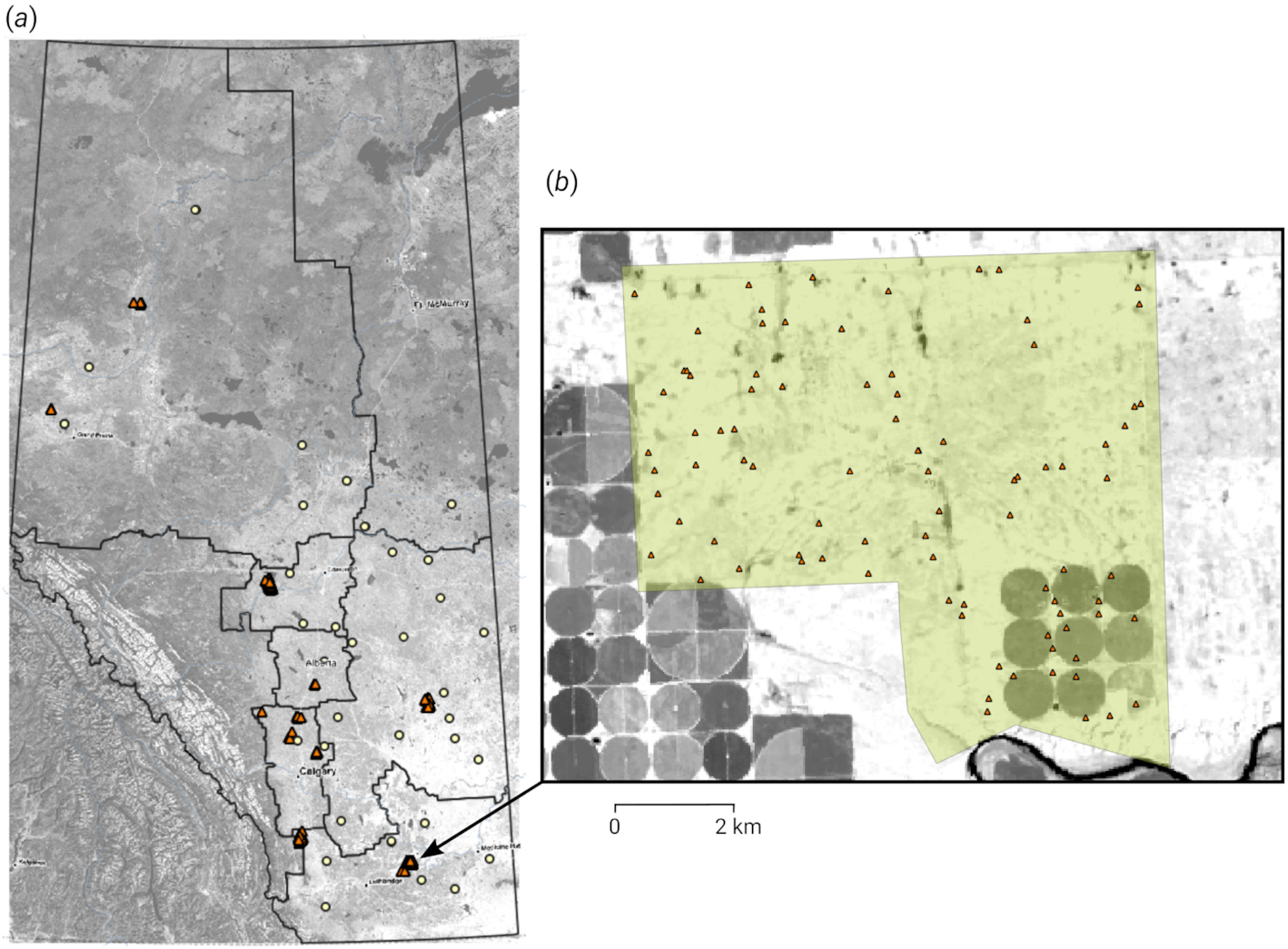
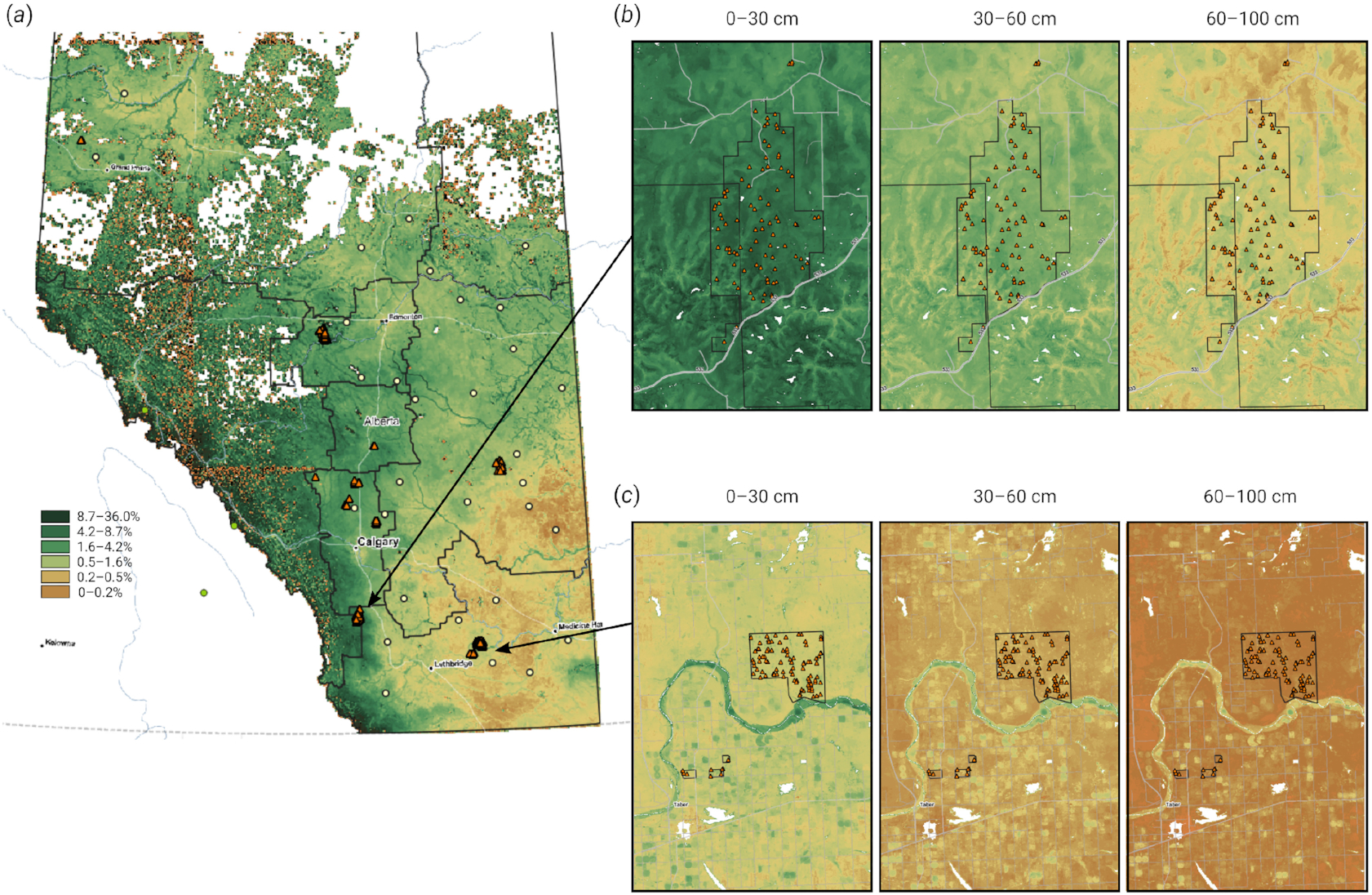
Roper et al. 2019) using a Carlo Erba NA 2100 Elemental Analyzer (Carbo Erba Strumentazione, Milan, Italy). Bulk density and coarse fragment content were also determined during laboratory analysis. The sampling locations across Alberta are illustrated in
Fig. 1.
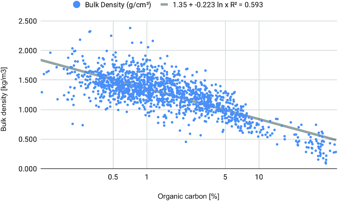
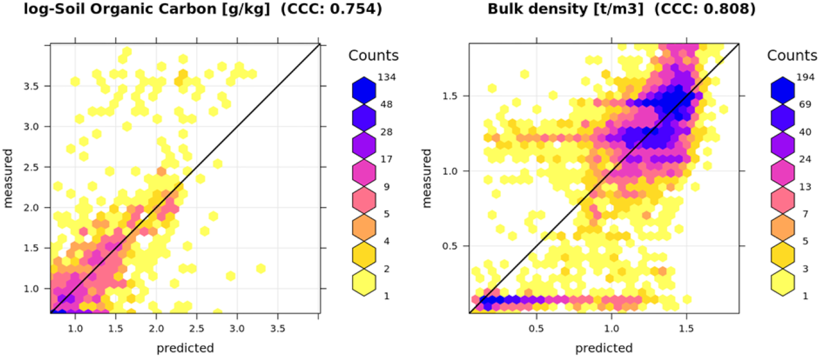
After laboratory analyses and data entry, all points were inspected for possible artifacts and gross errors. This was done by producing two-dimensional (2D) scatter and multivariate plots to detect potential outliers. Bulk density was available for a majority of soil samples. The remaining 10% of samples with missing values were estimated used a pedotransfer function shown in
Fig. 2 fitted locally using the AESA dataset.
Because the AESA SOC data were determined using loss on ignition and not dry combustion, we harmonized the loss-on-ignition values to avoid any bias in estimates
(Roper et al. 2019). For this we used the formula provided by
Jensen et al. (2018) that accounts for the clay content of soil:
where SOC is soil organic carbon content, LOI is soil organic carbon loss-on-ignition values, and CLAY is clay content.
2.2. Covariate layers
We focused on mapping SOC at spatial resolutions finer than recent Canada-wide work
(Sothe et al. 2022); hence, we prepared the covariate layers at spatial resolutions of 30 m. We prepared 180 covariates that can be grouped roughly into four themes:
•
Relief: we used the Advanced Land Observation Satellite (ALOS) Digital Terrain Model (DTM) of Alberta at 30 m
(Jaxa 2015).Terrain derivatives including standard morphometric and hydrological parameters at 30, 100, and 250 m spatial resolution were determined
(Behrens et al. 2018).
•
Organisms: we used the Moderate Resolution Imaging Spectroradiometer (MODIS) Enhanced Vegetation Index (EVI) long-term composites, PROBA-V Level3 Normalized Difference Vegetation Index (NDVI)
(Wolters et al. 2014) long-term monthly estimates, and Landsat Analysis Ready Data (ARD) 25th Percentile (P25), 50th Percentile (P50), and 75th Percentile (P75) images for spring and summer months (
Potapov et al. 2020;
Witjes et al. 2022).
•
Parent material: we prepared lithological units for Alberta based on the Bedrock Topography of Alberta Version 2
(Alberta Geological Survey 2020) downloaded from
https://ags.aer.ca/data-maps-models/data/dig-2020-0022; the units were converted to indicator maps for (1) colluvial deposits, (2) eolian deposits, (3) fluvial deposits, (4) glaciofluvial deposits, (5) glaciers, (6) lacustrine deposits, (7) glaciolacustrine deposits, (8) moraine, (9) fluted moraine, (10) stagnant ice moraine, (11) ice-thrust moraine, (12) organic deposits, (13) bedrock, and (14) preglacial fluvial deposits.
Preparation of the PROBA-V and Landsat long-term composites for recent years (2018–2020) required downloading the images from the GLAD Landsat ARD Tools (
https://glad.umd.edu/ard/) and then downloading long-term composites for four seasons (winter, spring, summer, and autumn months), removing snow cover and gap filling all missing pixels. The 7-band Landsat images produced a total of 168 GeoTIFFs (4 seasons × 3 percentiles × 7 bands × 2 years) that were then used as covariate layers. Detailed processing steps used to derive Landsat derivatives are available in
Witjes et al. (2022).
The rationale for using Landsat time-series composites for soil property mapping was as follows: although Landsat images do not penetrate soil and primarily reflect above ground vegetation (hence can not be used to measure SOC directly), we believe that by having full multi-year seasonal composites with three percentiles we can find key correlations among soil properties and the temporal signature of a pixel. Single-satellite images of a field can be strongly affected by crop-rotation effects, which are then reflected on predictions of soil properties. These crop-rotation effects most likely do not have anything to do with changes in soil properties, as many cropping systems’ above ground vegetation changes seasonally and abruptly with exactly the same soil properties. It is also important to emphasize that as data were used within a Machine Learning framework, primarily by fitting complex decision trees (e.g. Random Forest), each combination of crop rotation, seasonality, and other relationships that best fit the training data were determined. This assumption has worked in previous case studies (
Hengl et al. 2021,
2022a), with predictions not reflecting crop boundaries or similar patterns.
Although finer resolution spectral bands are now available, primarily thanks to the Sentinel-2 mission (up to 10 m spatial resolution), we focused on using Landsat as the key earth observation (EO) data for soil property mapping because our interest is the use of EO data to reconstruct historical SOC dynamics going back 10, 20, and 30 years.
After we prepared all covariate layers, training points were overlaid with 250 and 100 m resolution layers (climatic layers, MODIS LST, geological classes) and 30 m resolution layers (Landsat GLAD percentiles for bands for 2019 and 2020 digital terrain parameters) and then combined to produce a regression matrix with all covariate layers and target variables at different soil depths.
The whole of Alberta at 30 m as mosaics are images of 23 144 columns by 41 125 rows in the EPSG:3402–NAD83(CSRS)/Alberta 10-TM (Forest) coordinate system. The total data prepared for SOC mapping exceeded 200 GB. This means that a significant infrastructure is needed to process these data. Predictions were the most time-consuming task in the total workflow and were run in a high-performance computing environment (Intel Xeon Gold 6284R with 96 threads and 378 GB RAM) to avoid RAM limitations and delays.
2.3. 3D Ensemble Machine Learning
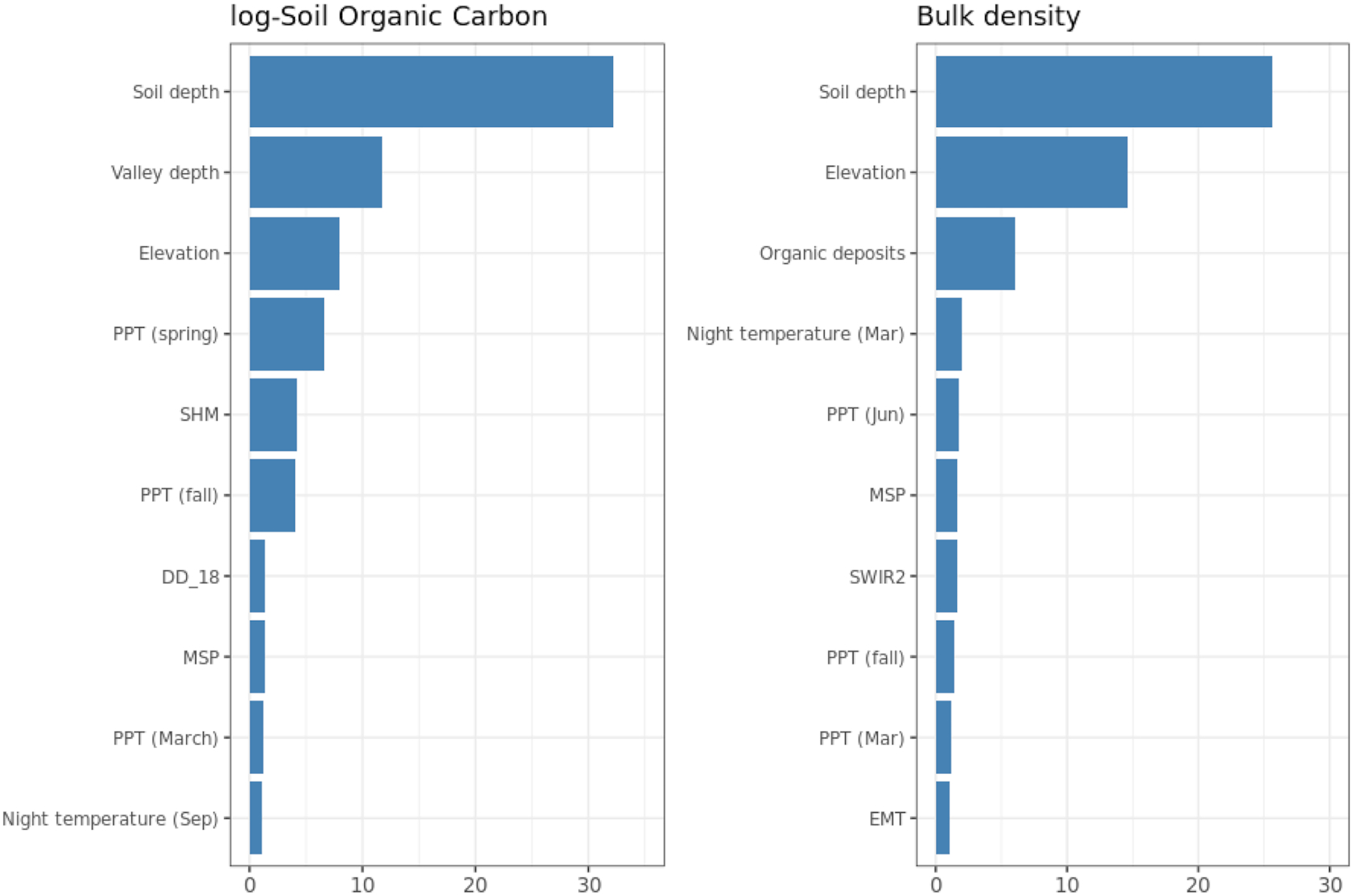
We used a three-dimensional (3D) Ensemble Machine Learning (3D-EML) framework to model spatial distribution in SOC and soil bulk density as explained in
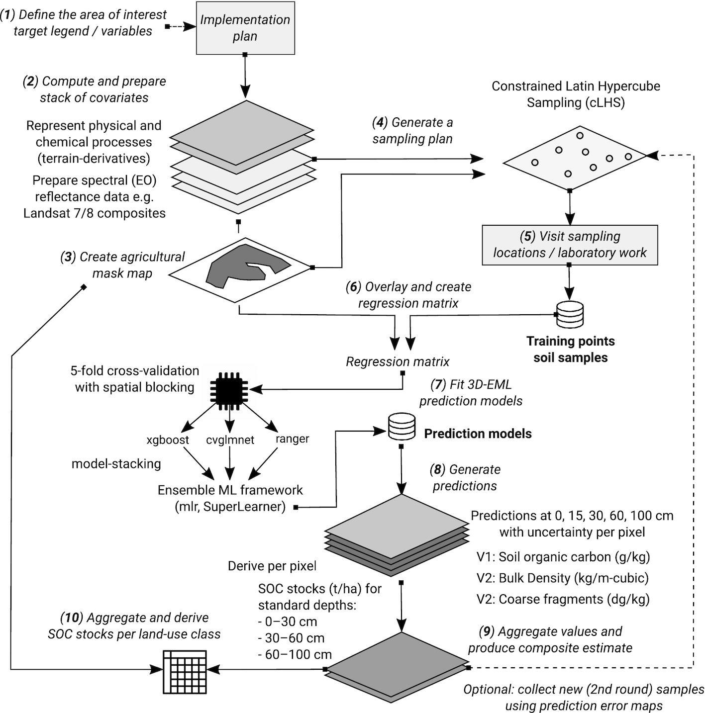
Fig. 3. We first defined an area of interest (agricultural mask) and prepared a list of covariate layers representing soil-forming factors (steps 1–3). We then used the covariate layers to design a sampling design (step 4) based on conditioned Latin hypercube sampling to ensure unbiased representation and minimal extrapolation space within the sampled farms
(Brus 2021). We next collected samples on the ground and carried out consistent laboratory analysis (step 5). The data from the samples were then quality-controlled and overlaid with covariate layers and used to build predictive models (steps 6–7) to map SOC content and bulk density independently (step 8).
After we produced predictions of SOC content and bulk density at depths 0, 15, 30, 60, and 100 cm, we derived aggregate estimates of the SOC stocks in depth increments of 0–30 cm (top-soil), 30–60 cm (sub-soil1), and 60–100 cm (sub-soil2) (step 9). The depth-wise estimates were modeled using a threshold as described in
Hengl and MacMillan (2019), where the values for the 0–30 cm depth interval were split into two values at 0 and 30 cm. These estimates were then crossed with the land use and soil type maps for Alberta to produce summaries per combination of classes.
The 3D-EML approach incorporated soil depth as a covariate, which enabled the prediction of a given soil parameter at any depth. The advantage of this approach over mapping each depth independently was that the total training data set could be maximized and variations in depth profiles could be accounted for in the model (
Hengl and MacMillan 2019;
Hengl et al. 2021). A disadvantage of this approach was that only the depth variable was modified and values of covariates at various depths were considered to be constant, which was a gross assumption.
Ma et al. (2021) compared the 3D predictive soil mapping with 2D approaches, including a combination with spline fitting of soil horizons and showed that 3D mapping produced comparable accuracy and was easier to implement as compared to 2D approaches that include multiple additional steps such as spline fitting/gap filling.
We ran model fitting and prediction in four phases, as implemented in the
mlr framework for Machine Learning in R
(Bischl et al. 2016). Standard four modeling steps included
1.
Hyper-parameters fine-tuning: we first determined mtry for ranger and XGBoost parameters by iterative fine-tuning;
2.
Feature selection: we subset covariates using random feature selection in mlr, which usually removes 30%–40% of covariates;
3.
Stacking: we used 5-fold cross-validation with spatial blocking (5 × 5 km) to generate a meta-learner;
4.
After the model fitting, we produced predictions and estimated the prediction errors (per pixel) by first fitting a quantile regression RF model using three learners and then derived root mean square percentage error per pixel using the
forestError package
(Lu and Hardin 2021).
We used EML rather than a single learner (e.g. Random Forest) for two main reasons: (1) it is a remedy for potential over-fitting and (2) in the case of variables with skewed distributions, it helps reduce overshooting effects (
Hengl et al. 2022a,
2022b). In the case of spatially clustered samples (this study also), spatial blocking (i.e. spatial cross-validation) during model training helped reduce potential over-fitting that can be significant (
Gasch et al. 2015;
Schratz et al. 2019). When points are based on probability sampling and regularly distributed across areas of interest, spatial cross-validation has produced over-pessimistic estimates of mapping accuracy
(Wadoux et al. 2021). In our case, because sampling points were clustered around selected farms, we needed to use spatial blocking (with 30 km tiles) during model training to prevent overfitting. Also, we assumed that to get a realistic estimate of the mapping accuracy for the whole of Alberta, we removed whole farms from training/validation.
Note also that we modeled the log-transformed variable for SOC and coarse fragments (both follow log-normal distribution) and then back-transformed after modeling. The rationale to work with the log-transformed variable is as follows: first, by log-transforming the target variable, we reduced the effect of very large SOC concentrations (e.g. high SOC in wetlands and similar areas that might result in low values being over-estimated); secondly, for the log-transformed variable, which then showed close to normal distribution, it was easier to interpret the root mean square error (RMSE) and visualize results.
2.4. Derivation of soil carbon stocks
Our main objective was to map SOC stocks in t/ha and not only SOC content. In principle, in predictive soil mapping, there are three main ways to derive SOC stocks from soil samples
(Hengl and MacMillan 2019):
1.
The 2D approach: estimate SOC stocks in t/ha for fixed depths, e.g., 0–30 cm, and then model and predict stocks or estimate SOC content and bulk density for each depth separately and combine to estimate total SOC stock.
2.
The 3D uni-variate approach: estimate SOC density in kg/m
3 for each soil depth (training samples) and then predict in 3D and aggregate to standard depth intervals
(Sanderman et al. 2018).
3.
The 3D multivariate approach: model and predict SOC content (g/kg), bulk density (kg/m3), and coarse fragments (dg/kg) independently in 3D and then aggregate to standard depth intervals and derive SOC stocks in t/ha.
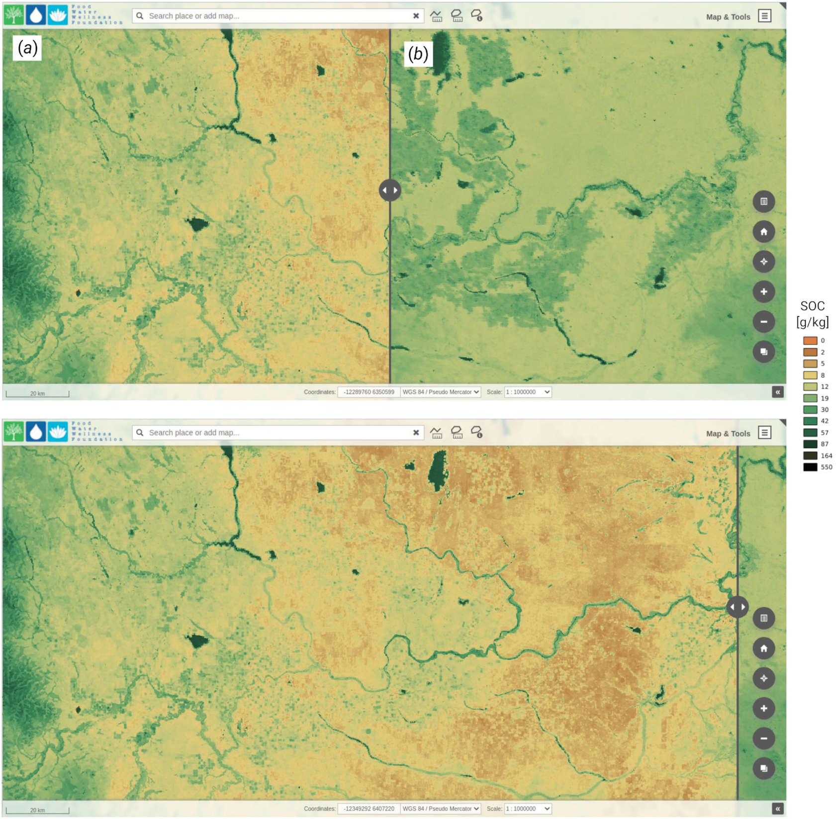
In this paper, we used a 3D multivariate approach as it enables relationships among soil properties and soil depth to be explicitly captured in the model. We derived SOC stocks from independently modeled and predicted SOC content (g/kg), bulk density of the fine earth fraction (kg/m3), and coarse fragments (dg/kg). After we produced maps for 3 soil variables at 5 depths (0, 15, 30, 60, and 100 cm), we aggregated values to standard depth intervals 0–30 cm and 30–100 cm and then derived SOC stocks for every pixel, including the uncertainty expressed as prediction error maps.
The SOC stocks in t/ha were derived using
Nelson and Sommers (1983):
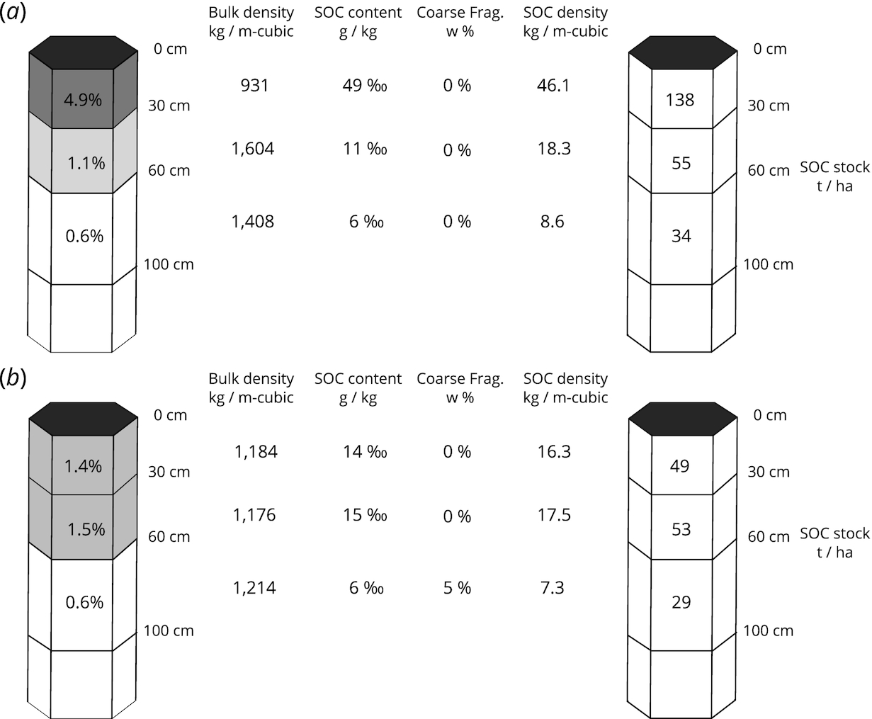
where OCS was soil organic carbon stock, ORC was soil organic carbon mass fraction in permilles, HOT was horizon thickness in m, BLD was soil bulk density in kg/m
3, and CRF was volumetric fraction of coarse fragments (>2 mm) in percent (
Fig. 4).
The uncertainty of estimating SOC stocks in t/ha for a 3D multivariate approach can be derived using composite prediction errors
(Hengl et al. 2014):
where
,
, and
are standard deviations of the predicted soil organic carbon content, bulk density, and coarse fragments (i.e. prediction errors), respectively.
2.6. SOC aggregation per land use and soil type
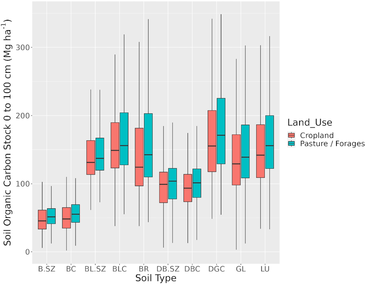
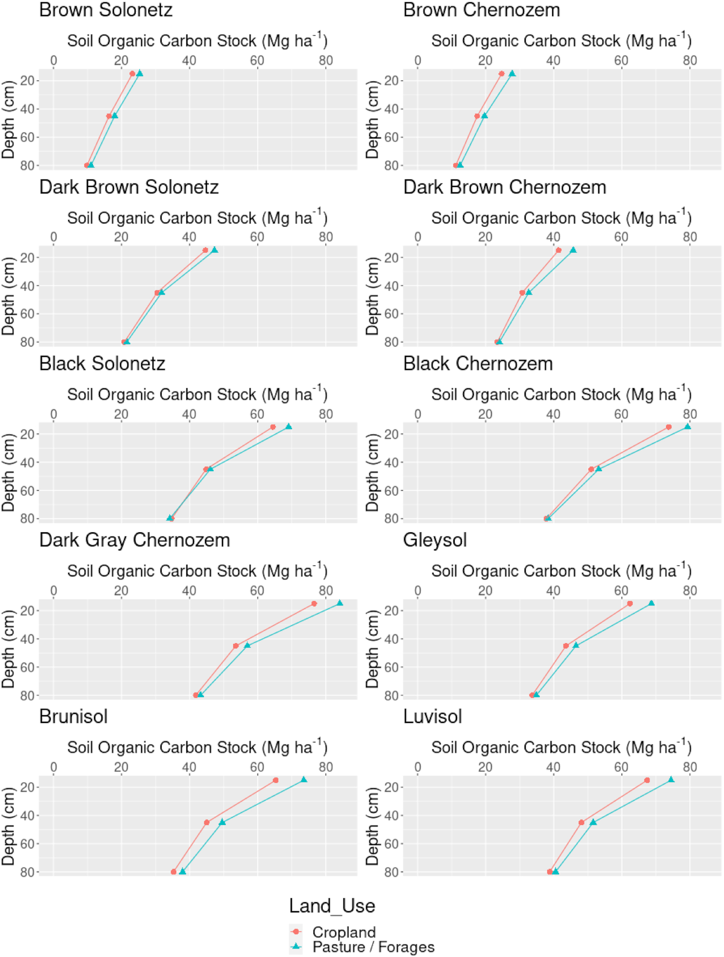
Following development of the predictive soil maps for SOC stocks to a depth of 1 m, the resulting data were used to assess the influence of land use and soil type on SOC stocks in Alberta’s agricultural region. To assess SOC stocks by soil type, soil type polygons from the Agricultural Regions of Alberta Soil Inventory Database were used
(Brierley et al. 2001). Land use was determined based on the Agriculture and Agri-food Canada Annual Space-Based Crop Inventory for Canada
(Government of Alberta 2022).
Soil types were assessed at the order level following the Canadian System of Soil Classification (CSSC), except for Chernozemic soils that were assessed at the great group level to account for the large climatic gradient that influences SOC stocks for Chernozems in Alberta. Solonetzic soils were also separated by the Brown, Dark Brown, and Black subgroups to account for this same climate gradient. The categories were as follows, according to the CSSC
(Soil Classification Working Group 1998) (with the World Reference Base classifications in brackets
(IUSS Working Group WRB 2014)): Brown Solonetz (Solonetz), Brown Chernozem (Kastanozem aridic), Black Solonetz (Solonetz), Black Chernozem (Chernozem), Brunisol (Cambisol), Dark Brown Solonetz (Solonetz), Dark Brown Chernozem (Kastanozem Haplic), Dark Gray Chernozem (Greyzem), Gleysol (Gleysol), and Gray Luvisol (Albic Luvisol). An important feature to note is that Gleysols are known to have high carbon stores (
Euliss et al. 2006), but they are distributed across all soil zones, so the values for this soil order were averaged across the climate gradient. Additionally, Gleysols are not extensively mapped as dominant soils in Alberta and many soil polygons contain Gleysols as minor soils.
Total SOC stocks from 0 to 100 cm were calculated for land use categories of forested, cropland, grassland, shrubland, and wetland (
Table 1). The forested land use category included conifer and broadleaf classes, cropland included all annual crop types, and grasslands included grassland, pastures, and forage land. SOC stocks from 0 to 100 cm, as a function of cropland and grassland land use categories, along with soil types, were then compared using a generalized least squares model with the
nlme package in R
(Pinheiro 2021). The interaction between soil type and land use type was tested, and it was significant (
p < 0.01). Assessment of other land use classes was not examined with the generalized least squares model to simplify the results and because the vast majority of the training data came from cropland and grassland land use types.
