Modelling the dispersion of infectious salmon anemia virus from Atlantic salmon farms in the Quoddy Region of New Brunswick, Canada and Maine, USA
Abstract
Pathogen dispersal from infected aquaculture sites into the surrounding ocean poses risks of infection to wild and farmed species, but is difficult to predict. This study aimed to build a framework using an ocean circulation and a particle tracking model in conjunction with a dynamic infection model and a virus inactivation model to simulate the dispersal of the infectious salmon anemia virus (ISAV) from Atlantic salmon farms. Simulated particles were released from hypothetically infected farms and advected by modelled currents. Inactivation of viral cohorts by ambient ultraviolet radiation and natural microbial communities was simulated during advection. Simulations showed that ISAV concentration varied spatiotemporally with the progression of the outbreak, current speed and direction, tidal elevation amplitude, and environmental decay. Connectivity among aquaculture sites varied in relation to seaway distances, though simulations showed that connectivity can also be asymmetrical between farm sites. Sensitivity analyses showed that the dispersal of ISAV was moderately sensitive to uncertainty associated with the viral decay model, highlighting the importance of obtaining accurate estimates of inactivation rates of ISAV. This framework provides an approach to simulate waterborne viral transmission that considers the biology and epidemic features of significance for pathogens and the dynamic conditions of the ocean.
1. Introduction
In the marine environment, most cultured finfish are reared in open-water net pens, where abiotic and biotic exchanges occur between the farm and the environment (Milewski and Smith 2019; Carballeira Braña et al. 2021). Pathogens and parasites carried by wild hosts migrating in the vicinity of aquaculture sites present a risk to the farm, as these can be transferred from wild hosts to farmed species (i.e., spill over) and amplified within the site, resulting in significant losses and costs to the industry (Grant and Jones 2011). These parasites and pathogens can then be spilled back into the environment, and in turn infect wild species, as well as farmed species located on adjacent sites (Ford and Myers 2008; Johnsen et al. 2021). Understanding the transport and dispersal of parasites and pathogens is thus important to assess the risk of disease transfer between wild and farmed conspecifics and guide implementation of efficient management practices that can reduce this risk or mitigate the impacts.
Progress in the development of biophysical models, which couple physical oceanographic models with epidemiological models of infectious agents, has allowed the emergence of new tools to characterize the transport and dispersal networks of pathogens and parasites in marine ecosystems (Page et al. 2005; Gustafson et al. 2007; Chang et al. 2014; Foreman et al. 2015a). Physical models can capture regional oceanographic conditions, such as currents, temperature, and salinity, and biophysical models link these parameters with pathogen or parasite dynamics to improve predictive abilities. For instance, models of outbreaks and spread of parasites like sea lice (Lepeophtheirus salmonis) have been expanded to include biological information, such as host density, life cycle stages, and vertical migration behavior (Johnsen et al. 2016; Salama et al. 2018; Cantrell et al. 2020a). As with parasites, the dispersion of pathogens, such as the infectious hematopoietic necrosis virus (IHNV), was also simulated by a hydrodynamic model wherein biological features were incorporated, including shedding rate, decay rate, and minimum infectious dose (Foreman et al. 2015b).
Most dispersal models of waterborne pathogens typically simulate one average or one worst case scenario of infection as a simplifying assumption without integrating the epidemic progression of the disease (Olivares et al. 2015; Foreman et al. 2015b; Cantrell et al. 2020b). Infection and viral shedding are dynamic processes, evolving over the course of an outbreak, with variable viral abundance released into the water, and dispersed in turn by ocean conditions. As infection worsens for individual fish, the population-level shedding rate will increase, up to a peak level from which it will decrease due to mortality, recovery, immunity, culling, etc. (Gregory et al. 2009; Mardones et al. 2009; Qviller et al. 2020). Viral inactivation in the marine environment is another important factor that impacts virus infectivity and disease transmission (Oidtmann et al. 2018). Ultraviolet (UV) radiation, native microbes in water, and temperature are some of the main factors leading to viral decay and eventual loss of infectivity with time (Tapia et al. 2013; Vike et al. 2014; Pinon and Vialette 2018). Temporal variation in infective particle release, either caused by natural or human intervention, needs to be captured by incorporating the infection dynamics of the outbreak and the inactivation processes into models, which enables more realistic scenarios of simulated pathogen transmission, better predictions of outcome, and, ultimately, more efficient management actions to be undertaken.
Many studies of infectious disease models in terrestrial animals have developed methods to integrate dynamic infection processes (Garner and Beckett 2005; Jenness et al. 2018). A notable example is the Davis Animal Disease Simulation model (DADS) (Bates et al. 2003), which was based on a susceptible-exposed-infectious-removed (SEIR) compartmental model (Kermack and McKendrick 1927). A later-developed version, the DTU-DADS-ASF (Danish Technical University - Davis Animal Disease Model -African Swine Fever) model (Halasa et al. 2019), was adapted to simulate infectious salmon anemia virus (ISAV) and IHNV infections within and between aquaculture sites in marine environments, with seaway distance as the primary determinant of waterborne pathogen transmission (Romero et al. 2021, 2022). This model provides an efficient tool to capture the dynamic evolution of infected fish numbers within a farm, which determines virus shedding and release. However, the impacts of the hydrodynamic oceanic environment and decay processes on pathogen dispersal have not been included. As a result, the simulations of spatiotemporal dispersal are limited due to the unaccounted-for effects of hydrodynamics and biological components on the virus.
Listed as a notifiable disease by the World Organization for Animal Health (WOAH), ISAV has caused severe economic losses in the Atlantic salmon (Salmo salar) aquaculture industry between the late 1990s and early 2000s, and it continues to create an economic burden (Gagné and LeBlanc 2018). These losses and potential pressures to the environment have led to significant efforts in salmon aquaculture regulation and management (Chang et al. 2014). Notably, the tidal excursion area and overlapping scales of water exchange for dispersing ISAV particles have been modelled with a 3-D tidal circulation and particle tracking model to support the establishment of bay management areas (BMAs) in southwestern New Brunswick (NB), Canada (Page et al. 2005). In these studies, the simulation of viral dispersal focused primarily on the development and application of physical models with recommendations to incorporate pathogen dynamics in future developments (Graham et al. 2007; Johnsen et al. 2014). In this study, we developed a four-module framework that includes hydrodynamics, ISAV infection dynamics, viral inactivation, and risk of infection for surrounding environments to simulate the transport and dispersal of ISAV from Atlantic salmon farms in the Quoddy Region of New Brunswick, Canada, and Maine, USA. The integration of these modules aims to bridge the hydrodynamic model and biological components of ISAV, especially the dynamic progression of an infection within an outbreak, which is currently lacking in virus dispersal models. By coupling the dynamics of a viral infection with hydrodynamic processes rather than simply using a given infection scenario, more realistic scenarios of the spatiotemporal virus distribution during an entire outbreak are produced.
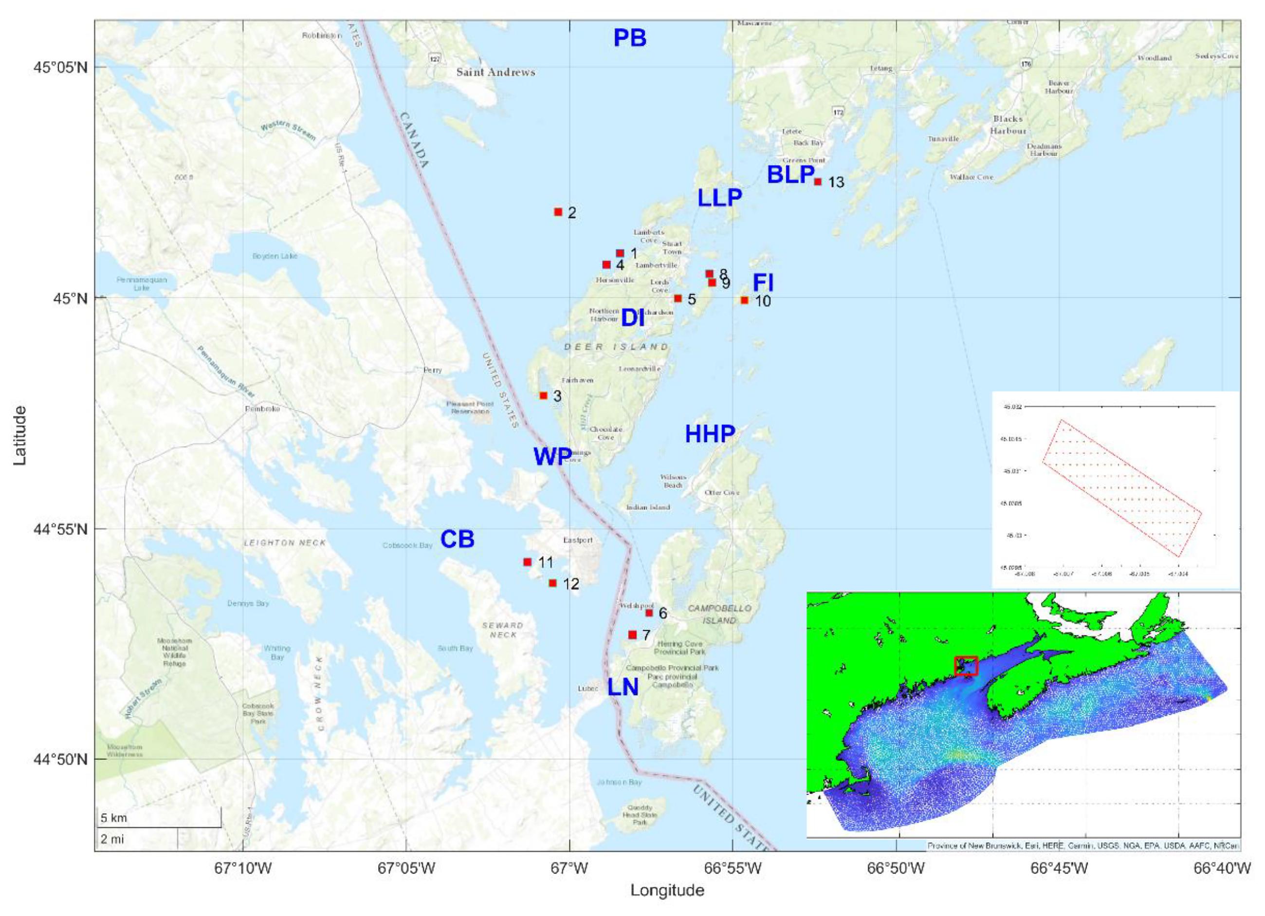
The Quoddy Region is an important salmon aquaculture area in the southwestern end of the Bay of Fundy and is bordered by the Canadian province of New Brunswick and the U.S. state of Maine (Fig. 1). It is a unique region with extreme tidal ranges (i.e., 7–8 m), freshwater inputs, and wind-driven surface currents (Trites and Garrett 1983; Greenberg et al. 2005). The first successful salmon farming in Atlantic Canada began in this region in 1979 (Anderson 2007; Chang et al. 2014). There are currently more than 50 salmon farming lease sites in the Quoddy Region, though less than half of the sites are active at any given time. Although ISA disease outbreaks in New Brunswick are currently a less severe issue than in past decades as a result of improved disease control strategies, the virus is still regularly detected, contributing to economic and environmental pressure in the region (Canadian Food Inspection Agency 2022). Hence, a better understanding of the dispersal of ISAV in the area is required for risk assessment of disease transmission and aquaculture management.
Fig. 1.
2. Method and data
A numerical modelling framework including four functional modules was developed to simulate the dispersal of ISAV. A schematic flowchart illustrating the different components of the framework is provided (Fig. 2). Each component is detailed in the following sub-sections. Parameters applied in the model are listed in Table 1. Assumptions made to run the simulations are summarized in Supplementary Information 1. The transport and dispersal of ISAV from the studied farms was simulated by the particle tracking module using the hydrodynamic variables retrieved from an ocean circulation model as inputs. The ISAV infection module simulated the evolution of a hypothetical outbreak in the index farm, i.e., the farm in which the initial infection develops, and output the quantity of virus shed at any given time. This output was used as an initial viral load carried by simulated particles from the particle tracking module. Then, the inactivation module simulated the attenuation of viral load as a function of the time exposed to marine microbes and UV radiation. The time series of viral load within each particle was further paired with the temporal position of particles simulated from the particle tracking module. Finally, the risk of infection module simulated the viral transport and dispersion in ambient water and to neighboring farms. Altogether, the framework models the epidemiological progression of ISAV outbreaks from farms, as well as the viral dynamic transport, dispersal, and infection risk in the surrounding environment. Thirteen farms representing a range of hydrographic conditions and connectivity were included in this study, and a simulation was completed independently with each of them as the index farm. All these farms are located in the migration path of Atlantic salmon post-smolts in the region (Lacroix et al. 2004; Quinn et al. 2022).
Fig. 2.
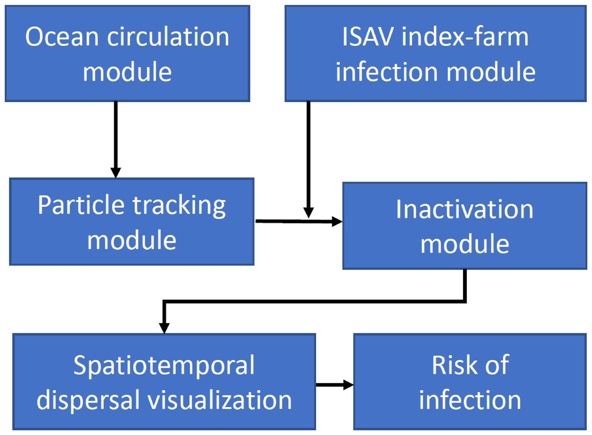
Table 1.
| Symbol | Parameter description | Value | Source |
|---|---|---|---|
| NT | Fish number in one farm | 300 000 | User defined based on local industry practice (personal communication) |
| W | Weight of each fish | 5 kg | User defined based on local industry practice (personal communication) |
| k | Transmission risk between fish | beta-PERT (0.8,0.9,0.99) | User defined to represent highly virulent variants |
| fl* | Input distribution of the latent period duration for individual fish | [0.000001,0.000001,0.0001,0.01,0.1,0.25, 0.339898,0.3] | (Romero et al. 2021) (Gregory et al. 2009) |
| fs* | Input distribution of the subclinical period duration for individual fish | [0.249995,0.50,0.25,0.000001,0.000001, 0.000001,0.000001,0.000001] | (Romero et al. 2021) (Gregory et al. 2009) |
| fc* | Input distribution of the clinical period duration for individual fish | [0.125,0.125,0.125,0.125,0.1 25,0.125,0.125,0.125] | (Romero et al. 2021) (Gregory et al. 2009) |
| N0 | Initial infected fish percentage | 3% | User defined |
| kuv | ISAV decay rate caused by UV | 4.85 × 10⁻⁵ J−1 m2 | (Garver et al. 2013) |
| kb | ISAV decay rate caused by microbiota | 4.18 day−1 | (Garver et al. 2013) |
| α | UV attenuation with water depth | 0.6396 m−1 | (Foreman et al. 2015b) |
| T | Minimum infectious dose of ISAV | 10 TCID50 mL−1 | (Gregory et al. 2009) |
| β | The amplitude coefficient of the normal distribution in eq. 2 | 27090335.11 | (Gregory et al. 2009) |
| μ | The mean coefficient of the normal distribution in eq. 2 | 14.18 | (Gregory et al. 2009) |
| σ | The standard deviation coefficient of the normal distribution in eq. 2 | 2.94 | (Gregory et al. 2009) |
Note:*The transition rate between infection stages (from susceptible to clinical) follows the distributions identified by *; each value represents the proportion of fish transitioning from one infection stage to the next, over the course of 8 days.
2.1. Ocean circulation module
A coastal ocean circulation model based on the unstructured-grid Finite Volume Community Ocean Model (FVCOM, Chen et al. 2012) has been implemented to simulate the dynamic physical oceanographic environment in Passamaquoddy Bay and adjacent areas (i.e., the Quoddy Region). A detailed description of the model can be found in Quinn et al. (2022), with some basic configurations summarized below. The FVCOM domain covers the Scotian Shelf, Gulf of Maine, and Bay of Fundy, including waters in and just outside of Passamaquoddy Bay (Fig. 1). The unstructured model mesh of FVCOM enables representation of the complex variation of bathymetry and coastlines in the region, with a horizontal resolution as fine as 25 m in shallow areas of the bay and along tidal channels, and as coarse as 11 km in deeper offshore areas; the largest mesh size in our area of interest is 1.2 km (Fig. 1). Vertically, the model comprises 20 geometrically spaced layers with finer resolution near the surface and bottom.
Comparisons of the physical oceanographic model's predictions were made against sea surface height measured from a tide gauge to the south of Passamaquoddy Bay and vertical temperature/salinity profile data from station Prince 7 of the Atlantic Zone Monitoring Program survey (https://www.dfo-mpo.gc.ca/science/data-donnees/azmp-pmza/index-eng), as well as overall regional patterns in surface residual currents, salinity, and temperature (Quinn et al. 2022). Further, the particle tracking model within Passamaquoddy Bay was tested against trajectories of GPS-equipped surface drifters (Quinn et al. 2022). Both analyses suggest that the model results can represent reasonably well the surface layer physical oceanography, ocean circulation processes, and particle trajectories in the studied area. More in-situ observations are needed to fully validate the model for operational applications, especially for the model capability of simulating vertical ocean dynamics.
In this study, hourly FVCOM outputs for the period between 1 May to 1 July 2018 were retrieved for analysis, as May–June is the period when wild post-smolt conspecifics are more likely to swim near salmon aquaculture sites in this area (Lacroix et al. 2004). Surface layer ocean currents in the study area from this model output are shown for ebb and flood tides on 1 June 2018 to demonstrate a general circulation pattern (Fig. 3).
Fig. 3.
2.2. ISAV index farm infection module
Temporal variation in the proportion of infected fish, along with the population-level viral shedding rate, were simulated by a dynamic infection module at one index farm at a time. The schematic flowchart of this module is shown in Fig. 4. The quantity of virus released by infected farmed salmon was determined by the number of infected fish in the farm, their size, and the viral shedding rate. The shedding rate is influenced by the level of infection of the fish, which follows a bell-shaped curve (Gregory et al. 2009). The peak of infection is usually observed at around 2–3 weeks post-infection, after which ISAV will eventually be cleared from the system of fish surviving the infection (Fig. 5).
Fig. 4.
Fig. 5.
2.2.1. Number of infected fish
When a disease outbreak occurs in an animal population, it generally goes through different stages from exposure to death or recovery. For the purpose of this study, we will consider the following four stages: latent (exposure to ISAV), sub-clinical (low viral load, not observable symptoms), clinical (period of illness with observable symptoms), and removed stages (i.e., immune, culled, or dead). To predict the number of fish at different stages, the infection spread within a farm was modelled by adapting the DTU-DADS-Aqua model (open source, available at https://github.com/upei-aqua/DTU-DADS-Aqua). For simplicity, we considered the entire farm site as one single cage. We pre-determined the total number of fish in farms, initial proportion of infected fish, and transmission risk coefficient according to the local farm features (e.g., number of cages at a site) and study purpose. Other features in the DTU-DADS-Aqua model, such as infection between net pens and farm sites and human intervention, including surveillance, disease detection, and depopulation, were not used for this study.
In this module, all fish are assumed to be susceptible to ISAV. Daily transmission of infection in a farm is determined by the transmission risk (k) and prevalence of infection in the farm, which is calculated by dividing the number of sub-clinically and clinically infected fish by the total number of susceptible fish (i.e., total number of fish minus removed fish).
The number of newly infected fish was calculated on a daily basis using a random binomial process, with the probability of infection φ (t) modelled as in Romero et al. (2021):where NSC(t) is the number of fish at sub-clinical stage, NC(t) is the number of fish at the clinical stage, NT(t) is the total number of all the fish that are on site, NI(t) is the number of removed fish, and t is the number of days post outbreak in the farm.
(1)
The transmission risk (k) is a user-defined parameter that was estimated using a beta-PERT distribution. The distribution was parameterized using an estimate of the minimum, most likely, and maximum values. In this study, these were defined as 0.8, 0.9, and 0.99, respectively, to simulate a hypothetical worst-case scenario, which could be caused by highly virulent ISAV variants. The infection progression was modeled by assuming an initial rate of infection of 3% among the fish population to start the outbreak (i.e., φ (0) = 3%). This rate is considered conservative as it is lower than the lowest infection rate that could be detected with current surveillance practices in New Brunswick, i.e., 5% when 20 animals are sampled (NBDAFF 2020). An average number of 300 000 fish per farm site was used (M. Szemerda, Cooke Aquaculture, personal communication 2021).
Newly infected fish were first counted as latent fish, then transferred to the next stages following predetermined durations, as described by Romero et al. (2021). Briefly, fish that transition to a new infection stage were assigned a number of days during which they remain in that stage based on the specified frequency distributions for the latent stage (fL), subclinical stage (fS), and clinical stage (fC), respectively. The frequency distribution indicated the proportion of fish that moves to the next stage over the course of 8 days and were taken from Romero et al. (2021) based on experiments conducted by Gregory et al. (2009), though they can be further refined with more experimental results.
The daily number of newly infected fish was redistributed into each of the 24 h of the day by linear interpolation to facilitate the calculation of virus-shedding rates on an hourly basis.
2.2.2. Number of released virus
The ISAV shedding rate varies over time as the infection progresses and was modelled by fitting a normal distribution function (eq. 2) to the laboratory data obtained by Gregory et al. (2009) as follows:where is ISAV shedding rate (in TCID50 kg−1 h−1) released from each individual infected fish i, on day t with a time interval of 1 h (1/24 days); t0i is the initial time that fish i was assigned to the latent stage; μ, β, and σ are the mean, amplitude, and standard deviation coefficients of the normal distribution function, respectively, which are obtained from the solver function in EXCEL® software, with solutions ofβ = 27090335.11, μ = 14.18, and σ = 2.94, and R2 = 0.99 (Supplementary Information 2). TCID50 is the amount of virus required to induce cytopathic effects in 50% of inoculated cultured cells (Virology Research Services 2019).
(2)
For each hour of the day, the total number of newly shed viruses released from the farm was estimated based on the number of infected fish, their size, and shedding rates as follows:where is the hourly population-level viral shedding rate (in TCID50 h−1) released from the infected farm at time t (h); N is the total number of infected fish at time t (h), as estimated according to eq. 1. The daily number of newly infected fish was calculated by multiplying the probability of infection φ (t) with the total number of susceptible fish in that day, then was interpolated into an hourly infected fish number to coordinate with the hourly particle release in the particle tracking module. Wi(t) is the size of individual fish (kg), which was set at 5 kg (i.e., size of the fish at harvest) to represent a worse-case scenario, though site-specific values can also be imputed in the model.
(3)
2.3. Particle tracking module
PTrack, a Lagrangian particle tracking model, was adapted to simulate the trajectories of viruses released from fish farms. This open-source package (https://github.com/SneakyNeko/PTrack) is specifically designed as an offline particle tracking tool for use with oceanographic output from FVCOM. Having the ability to carry out offline particle tracking increases the flexibility with which particles released at various locations and time periods can be tracked and can accommodate simulations of virus outbreaks from different farms and under different scenarios.
The PTrack model takes the ocean current variables simulated by the ocean circulation module as inputs to advect particles. The model has functionality to include additional movement of the particles themselves (e.g., swimming speed, sinking speed, etc.), although these were not considered in the present study, as viral particles are expected to disperse passively. In this study, to accommodate the diffusion characteristics of the ocean environment, 100 passive particles were released on an hourly basis from the studied farm for the duration of the outbreak (55 days). Each particle represented a cohort of infectious viruses with its initial load set as 100th of the initial virus amount shed from the farm at any given hour. The release points of the 100 particles were evenly distributed horizontally and randomly distributed vertically between 0 and 15 m (estimated depth of a cage) within the farm area. A random walk scheme was included in the model with both horizontal and vertical diffusion coefficients set at 0.1 m2 s−1, based on the turbulence characteristics of the study area (Page et al. 2014). The effect of the vertical diffusion coefficient was evaluated by repeating simulations using different values (see Supplementary Information 4).
After release, particles were subjected to passive drift following ocean circulation. The temporal interval of the PTrack module was set at 5 min. A 0.5 min temporal interval was also tested, with no significant differences observed in the particle movement over a period of 3 h (see Supplementary Information 3). A land avoidance scheme was applied in PTrack, such that when the next step of a particle is predicted to be on land, the particle remains in the current position until a new prediction is generated at the next step. Each group of particles was tracked for 24 h, which is long enough to cover the infectious state of ISAV particles (Jacquet and Bratbak 2003; Vike et al. 2014; D. Ditlecadet, unpublished data). The results of PTrack were saved for further coupling with the infection module (Section 2.2) and inactivation module (Section 2.4).
2.4. Inactivation module
Virions released into the marine environment are subjected to degradation caused by natural factors, such as microbial communities and UV radiation (Pinon and Vialette 2018). The combined effects of these factors determine the viability of the virus. Hence, an inactivation module was included in the dispersal model to address viral decay in the marine environment. Viral decay follows an exponential rate in seawater under natural sunlight (Garver et al. 2013), which was expressed as follows:where cΔt (TCID50 particle−1) is the virus load at any given time Δt elapsed after initial release from a fish farm (in days); c0t is the initial virus load per particle carried from the farm, as determined by the ISAV infection module (eq. 3), ; e −kbΔt is the viral decay with time exposed to the marine bio-communities, kb is the attenuation coefficient caused by bio-communities; e−kuvUVAB (Δt) is the viral decay due to the total ultraviolet A and B (UVAB) radiation during the period of Δt, and kuv is the corresponding decay coefficient. Because UV radiation attenuates with water depth, an exponential decay of UVAB radiation as a function of water depth was applied to estimate UV radiation at different depths (Foreman et al. 2015b). The cumulative UV exposure during the period of Δt was calculated by summing up the UVA/B radiation for all the time steps of the period, as shown in eq. 5:where UVAB (Δt) is the cumulative UVAB exposure at any given time Δt after initial release from a fish farm; n is the time step corresponding to Δt; UV0i is the sea surface UVAB radiance at time step i; zi is the water depth of the particle at time step i, which was simulated by FVCOM for each step; α is the attenuation coefficient of UVAB in local water. Because field data were not available for our study area, we adopted the value of α from the Discovery Islands, British Columbia, which is 0.6396 m−1 (Foreman et al. 2015b), though this value may be larger in our study area since the turbidity of water is likely larger in the Quoddy Region than in the Discovery Islands area.
(4)
(5)
In this study, the decay coefficients of kb and kuv were taken from experiments conducted on IHNV (Garver et al. 2013), and were set at 4.18 d−1 and 4.85 × 10⁻⁵ J−1 m2, respectively. These parameters were considered acceptable for ISAV based on the similar structures of the two viruses (i.e., enveloped RNA viruses), and preliminary results of lab measurements seem to support this assumption (N. Gagné, unpublished data). Nevertheless, to test the impact of decay coefficients, we performed a sensitivity analysis by varying kb and kuv by 20%.
UVAB exposure in sea surface was converted from UV index data in water surface, using the method introduced in Foreman et al. (2015b), (see Supplementary Information 5). UV index were taken from the closest available operational UV monitoring station, i.e., the Toronto, Ontario station (https://exp-studies.tor.ec.gc.ca). This station was at the closest latitude to the Quoddy Region, so it provides a comparable representation of the UV conditions in the study area, though in summer the UV index in the Toronto area is likely to be higher due to its slightly lower latitude (43.65 vs. 45.08, for Toronto and Passamaquody Bay, respectively).
2.5. Risk of infection module
To evaluate ISAV transport and dispersal patterns and estimate the infection connectivity among aquaculture farms, 13 active farms scattered in the Quoddy Region were selected as hypothetical viral release and receiving sites to represent an overview of the active farms in the area. Eleven farms were located in New Brunswick, Canada and two farms in Cobscook Bay, Maine, USA. Positions and spatial coverage of these farms were manually retrieved from high-resolution Google Earth® satellite images obtained in 2021 (Fig. 1). Together, these farm sites represent a range of hydrographic conditions (i.e., current speed and direction) and connectivity, with farms that are very close to one another (<500 m) to farms that are distant (∼25 km) and separated by islands. The depth of the fish cages deployed at these farms was set at 15 m (Chang et al. 2014), though this may vary among farms and can be adjusted as necessary in future simulations. For each farm, the number of 300 000 fish with a size of 5 kg (i.e., size of the fish at harvest) were selected to simulate a worst-case scenario in terms of fish density and biomass. These values can be adjusted as needed.
The horizontal viral transfer to other farms and fish in surrounding environments is referred to as the risk of infection herein. For ISAV, an exposure time of 1 h with a minimum infectious dose of 107 TCID50 m−3 was suggested to initiate an infection in Atlantic salmon (Gregory et al. 2009). Our unpublished laboratory results indicate that an exposure duration as short as 10 min can be sufficient if the variant is highly virulent (D. Ditlecadet, unpublished data). These criteria were adopted in this module as a threshold to estimate the risk of infection, i.e., during any continuous 10 min of the simulation period, when the virus concentration in the given space exceeded the threshold value of 107 TCID50 m−3, an outbreak in the receiving cage is triggered.
A second grid with equal-sized cells was implemented over the spatial domain to facilitate the calculation and visualization of viral concentration. The size of the second grid was arbitrarily chosen to be ∼135 × 47 m2 in the north and east directions, respectively. Secondary grid cells of different size/resolution may be used depending on the spatial coverage of the model domain, computational efficiency, and the purpose of the study (Supplementary Information 6). The viral concentration was calculated for each grid cell based on the virus load carried by each particle within the cells over 15 m depth to gain a general understanding of the infectivity of the virus over the studied domain. The spatial and temporal viral concentration maps associated with each index-farm were generated over the entire outbreak period based on the daily average viral abundances carried by the particles in each cell.
To demonstrate the spatial displacement of virus in the study area, particles with high viral load (HVL), i.e., greater than or equal to 1010 TCID50, were selected herein for distance calculation. With the infectious threshold of 107 TCID50 m−3, 1010 TCID50 is sufficient to make 1000 m3 of ambient water infectious to salmon (Gregory et al. 2009). This concentration was considered as a meaningful level of virus to have a significant impact in the open ocean environment. Dispersal distances of HVL particles were computed as the displacement between their travel positions and the center of their releasing farm. The mean dispersal distances of all HVL particles and the maximum value among them were recorded each day. To provide an overall view of HVL dispersal scale, an average value of daily mean distances for the entire outbreak period was calculated, as well as the average daily maximum distance. The standard deviation of all these daily mean distances, and daily maximum distances were computed to represent the diffusion of particles. The calculation of these distances was done for each farm and comparisons were made to illustrate variation among farms.
Infectious connectivity between farms was estimated as the likelihood of viral transfer from an infected farm to a naïve farm, using a method adapted from Foreman et al. (2015b). Briefly, given that the fish density in the farms is at least 1 fish m−3, arriving particles with viral load equal to or above 107 TCID50 were identified as infection sources. The connectivity between two farms (A and B) was quantified by the accumulated time when the viral loads of particles released from farm A and received by farm B exceeded the threshold value of 107 TCID50 and remained there for at least 10 min, the minimum time tested that caused an infection under laboratory conditions (D. Dilecadet, unpublished data). Then, the time was normalized as the percentage of the total outbreak time. Higher percentages indicated higher connectivity.
To better understand the different connectivity between specific farms, a statistical analysis of ocean current vectors at the associated farms was conducted. Based on the traditional wind rose method widely used in meteorology (Pereira 2022) and on current vectors extracted from the FVCOM output, a “current rose map” was constructed to create a direction intensity histogram for selected farms for the study period between 1 May and 30 June 2018.
3. Results
3.1. Dynamics of infection and shedding rate
Based on the modeling scenario defined in the ISAV index farm infection module, the proportion of infected fish increased rapidly after 5 days post infection and reached its peak after 30 days. At this time, most fish (99.9%) had been infected (Fig. 5). In the following days, the infected proportion remained steady, while infected fish experience sub-clinical and clinical stages, and eventually reached the final stage, where they were removed from the population.
The shedding rate at the index farm started soaring after 14 days post infection, increased rapidly in parallel with the proportion of infected fish, and peaked at day 37, where it was estimated at about 2.1 × 10¹² TCID50 h−1. Then, it dropped sharply and was near zero on day 55, i.e., the end of the outbreak (Fig. 5). There was a delay of 7 days between the times of the peak proportion of infected fish (i.e., 100% infected fish) and the peak shedding rates (i.e., when viral load is at its highest in the population).
3.2. Inactivation rate
ISAV was rapidly inactivated in sea water (Fig. 6). Inactivation by ambient microbes only had a relatively moderate effect; viral survival rate dropped to 1% within 26.4 h. When both UV radiation and microbial effects were included, inactivation happened much quicker. With the average UVAB radiation value of May and June 2018 in our studied area, it took less than 1.6 h for 99% of virus to lose infectivity at a water depth of 0 m and less than 4.9 h at a water depth of 2 m. After 24 h, there was hardly any infectivity left, and the fractional survival rate of virus was below 10−10 both on the surface and at the 2 m depth (Fig. 6). Therefore, out of consideration for computational efficiency, we assumed that 24 h was long enough to represent the full lifespan of ISAV in the marine environment. This lifespan was used in the PTrack module to track the dispersion of viral cohorts after release from farms.
Fig. 6.
To assess the robustness of the Inactivation model to uncertainty in kuv and in kb, we performed a sensitivity analysis by modifying these parameters by ± 20%. A 20% change in kuv changed the time to reach 1% survival rates between 1.3 and 1.9 h, which corresponds to about 19% variation compared with the original value of 1.6 h. If only considering the microbial effect, with a ±20% change in kb, the time taken to reach 1% survival rate ranged between 22.0 and 33.1 h without any UV radiation, which corresponds to a difference of about 16.7 and 25.4% compared with the original value of 26.4 h.
3.3. Viral concentration maps
Daily dispersal maps with average viral load over the top 15 m of the water column were produced for Farm 2 following a simulated outbreak for illustrative purposes (Fig. 7; see Supplementary Information 7 for the other farms simulated in this study). The concentrations of viral plumes evolved with the shedding process. On day 10, the viral load of the plume was in the order of 102 to 106 TCID50 m−3 and covered a 2 km circular area around the farm site (Fig. 7a). On day 20, particles had dispersed further out from the site and formed a roughly triangle-shaped pattern, with higher concentrations in proximity to the site than along the edges of the triangle (Fig. 7b). While some lower-concentration clusters dispersed east and south and reached the Western Passage (WP) area, the main direction of dispersal of clusters released from this site was eastward, with some moderate- to low-concentration clusters entering Little and Big L'Etete Passages (LLP and BLP, respectively). On day 30, the high concentration area extended well outside the farm site. Some medium to low concentration plumes spread in the northeast direction beyond the 5 km radius circle (Fig. 7c). On day 40, close to the peak time of shedding rate, the viral concentration in the proximity of the farm site reached an even higher level of 106 to 108 TCID50 m−3, while the dispersal scale was reduced markedly, with few low-concentration cohorts on the edge of the plume (Fig. 7d). On days 50 and 55, the overall viral concentration of the plumes decreased, while the shape of the plumes was similar to the one observed on days 20 and 30. All figures showed that high concentration plumes above 107 TCID50.m−3 mostly occurred very close to the farm center, where they hardly reached a half of the 2 km radius, i.e., 1 km from the center (Fig. 7).
Fig. 7.
3.4. Dispersal distance of high viral load (HVL) particles
The overall mean and maximum dispersal distances of HVL particles (viral load over 1010 TCID50 particle−1) from all the selected farms were about 0.3 km and 2.5 km, respectively, though these varied considerably among farms (Fig. 8). HVL particles from farms near Lubec Narrows (Farms 6 and 7), the Fundy Isles (Farms 8 and 9), and Eastport, Maine (Farms 11 and 12) showed longer distances (Fig. 8). HVL particles from Farm 6 displayed the longest distance, with mean and maximum values exceeding 0.6 and 6.3 km, respectively. Dispersal of HVL particles from farms located around the Deer Island coast (Farms 1 to 5) were relatively short, with mean distances of less than 0.2 km and mean maximum distances below 1.5 km. Farm 5 showed the shortest travel distances, with mean and maximum distance values of about 0.1 km and 0.9 km, respectively. Farm 13, located near Big L'Etete Passage (BLP), was close to the average distances calculated when including all the farms.
Fig. 8.
3.5. Infectious connectivity between farms
Results showed that most farms have an infectious connectivity lower than 5%, with an overall tendency for farms separated by shorter seaway distances to exhibit higher connectivity (Fig. 9). For instance, Farms 1 and 4 are separated by a seaway distance of 0.6 km and had a predicted connectivity above 50%, whereas Farms 11 and 12 are separated by a seaway distance of 1.3 km and had a predicted connectivity of 20%.
Fig. 9.
Values on the diagonal of Fig. 9 represented the “boomerang” effects of infectious particles on the release farms themselves. Farm 6 had the lowest value at about 48%, meaning that for 48% of the outbreak time, infectious particles remained at or returned to Farm 6. In contrast, Farms 1, 3, 4, 5, and 10 showed higher retention time, with infectious particles remaining at these farms for over 80% of the entire outbreak time (Fig. 9).
The reciprocal connectivity was also variable between farms, varying from symmetrical to asymmetrical (Fig. 9). For instance, connectivity between Farm 1 and 4 was strongly symmetrical, with rates of 53%–56% in either direction (i.e., Farm 1 to 4 or Farm 4 to 1). In contrast, connectivity of Farm 5 was strongly asymmetrical with both Farm 8 and Farm 9, with rates of 32%–33% from Farm 5 to Farm 8 or Farm 9, but only 2%–3% in the reverse directions.
For illustration purposes, the current vector statistical analysis was performed for two groups of farms (Farms 5, 8, and 9 and Farms 1 and 4) to better understand their reciprocal connectivity (Fig. 10). Two different patterns in terms of current directions along with the direct routes between farms were demonstrated. This analysis suggested that Farms 8 and 9 are directly downstream of Farm 5 (Fig. 10a). However, Farm 5 is seldom downstream of Farms 8 and 9 (Fig. 10a). In contrast, Farms 1 and 4 are directly upstream and downstream of each other, respectively, and thus water exchange is symmetrical between them (Fig. 10b).
Fig. 10.
4. Discussion
In this study, we developed a numerical modelling framework to simulate the dispersal of ISAV following a hypothetical outbreak at selected salmon farms in the Quoddy Region by coupling physical ocean circulation and particle tracking models with biological models, including a dynamic infection module and a virus inactivation module. Using this framework, viral dispersal maps for farms were produced, which indicated that the concentration level of ISAV varied spatiotemporally with the progression of the outbreak, hydrodynamic conditions, and environmental degradation. The risk of infection transmission was estimated in the ambient water and between farms by the simulation of dispersal distances of infectious cohorts and farm connectivity. The impacts of farm locations on viral dispersal distance and connectivity levels were identified, which could provide valuable information for risk assessment and aquaculture management. Below, we discuss the capabilities of the model along with its limitations and possible future development.
4.1. Impacts of hydrodynamics on ISAV dispersal
Since waterborne virus are expected to disperse passively, the physical movements of ISAV are substantially impacted by local hydrodynamic conditions. As a result, the spatial dispersion scales, as well as the concentration of ISAV, changed dramatically during the progression of the outbreak. For instance, while the viral concentration reached a peak around day 40, the dispersal scale was reduced markedly at that time instead of expanding. This change corresponded with the decreased tidal elevation amplitude at this time, modulated by the spring-neap tidal cycle, which was at a low level between days 35 and 40 post-outbreak (Supplementary Information 8). This indicates that, in tidally mixed systems, variation of tidal amplitude can be used to assist the prediction of viral dispersal, though many other factors also need to be considered, such as vertical mixing and turbidity caused by tidal dynamics (Davies et al. 1995; Pinon and Vialette 2018).
Current speeds are important for the dispersal distances of particles. As demonstrated in our results, particles from farms surrounded by high-speed currents had longer travel distances. In our simulations, the mean maximum dispersal distance of HVL cohorts was about 2.5 km for all selected farms, while it was about 6 km for Farm 6 as it is subjected to the fastest currents among the farms used in these simulations. Page et al. (2005) estimated that the maximum displacement of modeled ISAV particles from salmon farms located along southern Grand Manan Island, NB, varied between 2.3 and 13.9 km on a single tidal excursion, depending on site. This was longer than what we obtained in our simulations, possibly because they did not account for the viral shedding dynamics and environmental decay in their simulations.
Our modeling results also indicated that the mean displacement of HVL cohorts was about 0.3 km from the studied farms, providing a preliminary reference for future field work on ISAV. Field studies conducted in Norway revealed that ISAV RNA could be detected within a farm site experiencing an ISAV outbreak, but not in downstream water samples collected 70-100 m away (Løvdal and Enger 2002). This suggests that the dispersal of ISAV may be lower than predicted by our modeling effort. However, the number of infected fish, fish size, outbreak season, current speed and direction, and UV radiation condition were not reported in their study area, which can all impact the dispersion and concentration of ISAV dramatically, and need to be considered when comparing results among different ecosystems and seasons.
In our study, each farm was treated as a homogeneous unit, without considering the layout of individual cages and associated cage drag on hydrodynamics. In reality, farm areas are exposed to unique local oceanic conditions, as the flow speed and direction can be impacted by existing cage systems (Wu et al. 2014, 2022; Rickard 2020), which may affect viral dispersal. The viral transmission risk between cages likely varies as well, depending on the layout of cages (Romero et al. 2021). Our assumption of a single unit could be improved by coupling the dynamics of infection between cages model developed by Romero et al. (2021). Oceanographic conditions of hourly outputs from the FVCOM model were used to drive the particle tracking and reduce computing time of the simulations. Although this resolution has been generally used in tidally dominated areas (e.g., Foreman et al. 2015b; Quinn et al. 2022), it may need to be refined. Notably, the stability of particle tracking results in relation to the frequency of the circulation model outputs should be validated further. In addition, the temporal resolution of the particle tracking module can impact the stability of the simulation as well and need to be considered. Our preliminary tests indicate that, within short tracking periods (e.g., 3 h), differences in particle trajectories between temporal steps of 30 s and 5 mins were relatively small (Supplementary Information 2). This indicates a limited impact of 30 s interval setting on our ISAV trajectories since viral lifespan is predicted to be short (i.e., <3 h).
The random walk scheme in the PTrack module includes smaller scale turbulent mixing with preset homogeneous horizontal and vertical diffusion coefficients. However, model outputs of the FVCOM suggest that in parts of our study area, vertical diffusion coefficients may be smaller than horizontal diffusion coefficients (Supplementary Information 4). A comparison of the particle trajectory performed using two different vertical diffusion coefficients showed that the dispersal scale of particles was larger when the vertical diffusion coefficient was set to 0.01 m2 s−1 compared to 0.1 m2 s−1. Considering that most of our selected farms are scattered in the higher vertical diffusion area based on the FVCOM estimation, a vertical diffusion coefficient of 0.1 m2 s−1 was used for this study, although vertical turbulences around farms 1, 2, 3, and 4 are likely much lower than for other farms. Introducing spatially variable vertical diffusion coefficients to the particle tracking model may improve the accuracy of particle trajectory simulations (Stucchi et al. 2011).
4.2. Dynamic infection and viral shedding
One key component of the current modelling framework is that it accounts for the progression of an infection within an index farm, which integrates factors including the number of susceptible fish, fish size, virulence of variants, prevalence of the initial infection, and shedding rates at any given time. These factors determine the amount of virus shed in surrounding waters throughout the outbreak, which directly impacts the dispersal predictions (Salama and Murray 2011; Foreman et al. 2015a, 2015b). These settings can be adjusted according to different scenarios, providing flexibility for the implementation of this framework. In our study, all the fish were assumed to be susceptible to ISAV, with an initial abundance set to 300 000 per site in all farms and an average fish weight of 5 kg (i.e., market size) to mimic a worst case scenario. In practice though, information on fish stocking and production cycles can be used to represent specific scenarios, and to harness the full potential of this framework for quantifying the role of fish density in ISAV transmission to neighboring farms and ambient water. For instance, fish are currently less than 200 g at the time of stocking in our study area. As such, ISAV outbreaks occurring in smaller fish would result in reduced viral concentrations shed into the water, resulting in a reduced risk of infection relative to the values estimated in the present simulations.
The transmission risk between fish is a stochastic process and user-determined parameter in this model, which can be modified in accordance with the virulence of different variants and environmental conditions (Romero et al. 2021). The parameters used in this study to simulate the transmission risk of ISAV between fish were based on a beta-PERT (0.8, 0.9, and 0.99) distribution and represent a highly virulent scenario. This setting controls the entire outbreak time, which lasts for about 2 months in our simulation. The transmission risk may be lower than this for moderate variants, requiring different values for the beta-PERT function.
Estimating the shedding rate of ISAV-infected salmon is a complex task. Fish size, genetics, overall health status, temperature, and virus variants are all factors potentially influencing the virulence of the infection and the shedding rate (Madetoja et al. 2000; Hershberger et al. 2010; Purcell et al. 2016). In addition, dead fish remaining at the bottom of the net pen could release ISAV for some time, though the infectivity of the viruses released by dead fish is unknown (Wargo et al. 2017). In this study, fish were assumed to be removed once they were dead, and as such, dead fish did not release any ISAV in our simulations. The data we used to simulate individual shedding rates were extracted from the experimental work of Gregory et al. (2009). Their results, obtained from a highly infectious ISAV variant, were based on polymerase chain reaction (PCR) detection of virus and converted to equivalent TCID 50 mL−1 kg−1 using a calibration curve. Since the quantification of RNA of ISAV does not discriminate between infectious virions and RNA (Vike et al. 2014), the shedding rates used in this module may be overestimated. In addition, the Gregory et al. (2009) did not specify if they accounted for the initial concentration of ISAV at the beginning of their shedding experiments, which could also lead to an overestimation of shedding rate. Hence, additional experiments would be beneficial to optimize the estimation of ISAV shedding rates.
In our current simulation, human interventions, such as vaccination and de-population, were not included, providing the perspective of a worst-case infection scenario. For highly virulent variants, management actions would likely be taken as soon as clinical signs and/or unusual rates of mortalities are observed, such as culling the fish. As a result, the actual outbreak time may be much shorter that was simulated in this study. The infection module can be adapted to include human interventions (Romero et al. 2021), depending on the research purpose.
Exposure and infection resulting from multiple farm outbreaks were not accounted for in this study. During a disease outbreak, multiple farms can be infected and shed simultaneously, and this can have a cumulative impact. This scenario could be simulated using this framework with a few modifications.
4.3. Impacts of environmental parameters on ISAV inactivation
Waterborne viral cohorts are exposed to ambient seawater conditions that can affect their viability outside of the host, and, as a result, affect how far they can be dispersed by currents. In this study, we modelled the inactivation of ISAV in seawater as a function of both bacterial degradation and UV radiation. Sensitivity analyses indicated that the inactivation model was moderately sensitive to the uncertainty in these parameters; that is, a perturbation of ±20% changed the time to 99% inactivation time by about ±20% of the nominal value. Hence, there is a need to obtain accurate estimates of inactivation rates of ISAV along with the environmental conditions that are likely to affect these rates, such as UV radiation, to accurately predict the dispersal of ISAV in seawater.
In this study, we used the inactivation parameters that were derived by Garver er al. (2013) for IHNV, assuming that the viability of ISAV was similarly affected by UV radiation and bacterial degradation. The model predicted that infectivity would decrease rapidly and be near zero after about 3 h. This is consistent with the results of laboratory studies performed using natural seawater that showed a near total loss of ISAV infectivity within 3 h following an exposure to ambient UV radiation (Vike et al. 2014; D. Ditlecadet, unpublished data). In contrast, using sterilized water, Nylund et al. (1994) reported a viral lifetime of 20 h for ISAV, suggesting that bacterial degradation of ISAV is significant in natural seawater. Consequently, virions apparently lose their infectivity within a relatively short timeframe, limiting the risk of transmission, as shown by our modelling results.
The model we used to estimate the effects of UV radiation on the viability of ISAV also requires measurements of UV radiation in the region where the modeling was conducted, as well as the UV attenuation coefficient with water depth. In this study, the UV index was from the city of Toronto (Canada), the closest operational UV monitoring station. The relatively higher latitude of the Quoddy Region is expected to correspond to a lower UV index than Toronto, especially in the summer, when a 3% difference can exist during May to June, according to the numerical forecast data from Environment and Climate Change Canada (https://exp-studies.tor.ec.gc.ca/). Hence, the UV radiation used in our simulation may have been overestimated by approximately 3%. For the UV attenuation coefficient with water depth, we used the value derived by Foreman et al. (2015b) based on measurements conducted in the Discovery Islands, British Columbia. In addition, differences in cloud coverage between regions were not accounted in the present analyses, which could have biased the level of UV radiation predicted to reach the surface of water. UV attenuation rate with water depth is heavily modulated by the dissolved organic matter (DOM) content, sedimentation, and plankton concentration of the water, which themselves have strong spatial and seasonal variations (Häder et al. 2015). The interaction of these impacts may change the dispersal of ISAV, adding uncertainties to the modelling results. Obtaining UV measurements and attenuation coefficient for the studied area that also accounts for regional variation in cloud coverage would greatly reduce uncertainty, resulting in a more robust model.
The inactivation module can be adapted to account for additional environmental factors that may affect the viability of viruses, such as water temperature and salinity (Tapia et al. 2013). In our study, the inactivity coefficients derived at 10 °C was adopted (Garver et al. 2013). We did not account for changes in water temperature, which varied between 7 and 10 °C over the course of our simulation, though the viability of ISAV was expected to vary by less than 8% over that range of water temperatures (Tapia et al. 2013). Nevertheless, further effort is required to model the effect of water temperature and other environmental conditions on the viability of ISAV in local water.
4.4. Farm connectivity and aquaculture management
Connectivity analysis is useful to identify which sites have a higher potential of affecting other sites. Our simulations indicate that the potential for connectivity risks between several close farms could be higher than 50%. Without efficient early stage disease surveillance and response, infection transmissions are likely to occur among these farms. This supports the importance of industry adherence to stringent surveillance programs and disease management practices to minimize risks to nearby farms and wild species (NBDAAF 2020). Meanwhile, it should be noted that the dynamics of the outbreak and shedding rate may vary with the ISAV variants based on their virulence. For infections induced by highly virulent ISAV variants, actions are usually taken in earlier stages to reduce the risk of transmission between farms, and their impact.
Seaway distance has frequently been used in previous studies to estimate the connectivity among farms (Aldrin et al. 2011; Gautam et al. 2018; Parent et al. 2021). Our results indicate that accounting for seaway distance is essential when predicting connectivity between farms, given that most farms separated by short seaway distances showed high potential infectious connectivity. However, our connectivity and current vectors analyses indicate that it is also important to consider current directions due to the asymmetrical connectivity between some farms. For instance, we show that Farm 5 likely had a significant impact on Farms 8 and 9, while the reverse was less probable. These results further highlight the importance of considering ocean circulation to understand viral transmission and connectivity among farms rather than just distance alone (Gustafsen et al. 2007; Foreman et al. 2015b), supporting previous findings that farm location can play a vital role in disease transmission (Page et al. 2005).
The modelling results also indicated that the two farms located in Cobscook Bay, Maine, were connected to several farms located in Canadian waters, though at a very low level. This is a reminder that what happens in one jurisdiction might affect salmon farms in other jurisdictions and emphasizes the importance of bilateral coordinated efforts to improve aquaculture management.
In addition, modeling the connectivity between farms may provide some insight into the flushing ability of the index farm, as the diagonal line of that matrix is an indicator of the retention time of infectious particles at those sites. As the shedding dynamics were the same for all farms in our simulation, farms with high flushing ability can flush away the infectious particles in a relatively brief time, resulting in a reduced retention probability. For instance, Farm 6 had the lowest retention time, and dispersal distance of HVL particles from Farm 6 was the longest among the 13 farms. Such information can be useful to study the local environmental impacts of aquaculture activities, such as dispersion and deposition of fish feces and leftover food (Law and Hill 2019).
4.5. Future perspectives
It is always challenging to measure virus transmission in a real and dynamic marine environment due to the difficulty of conducting a large-scale field survey at the time of a virus outbreak. The current modelling framework provides a useful tool to understand such processes. The modelling results can be further validated and improved by integrating results of more laboratory and field work, including spatial epidemiological data, e.g., eDNA sampling and detection of pathogens and parasites in water samples, at a regional scale (Abbott et al. 2021).
By coupling the infection dynamics with other modules, this framework allows scenarios of outbreaks at earlier and later infection stages, as well as such management interventions, like culling and vaccination, to be simulated independently. Seasonal variations can be estimated by simulating outbreaks occurring at different times, especially with more environmental parameters involved. The spatial and temporal distribution of virus can also be simulated with this framework, allowing us to estimate the potential of infection in an area following one or multiple outbreaks. This is a key component to assess the risk of ISAV transmission not only to other farms, but also to wild Atlantic salmon that may transit through these sites. For instance, the migration paths and swimming behavior of Atlantic Salmon post-smolts were studied in the area where we simulated the dispersal of ISAV in this study (Lacroix et al. 2004; Quinn et al. 2022). With such information, this framework can be applied to estimate the potential exposure of wild fish to ISAV and assess the risk of farm-to-wild fish disease transmission.
The connectivity matrix obtained in this study may also prove to be a valuable tool for management purposes to guide site location and deployment of monitoring resources, as was done for sea lice in Scotland (Adams et al. 2016). For instance, the creation of BMAs in southwest New Brunswick was implemented in 2005 as part of the efforts to control ISAV in this area (Page et al. 2005, F. Page personal communication). Although the models used at the time to define these areas were relatively simple (i.e., an M2 (semidiurnal lunar tidal constituent) circulation model, ballpark estimates of viral inactivation time scales, no consideration of time-dependent shedding), the estimated displacement scales were considered reasonable and somewhat precautionary estimates for the geographic area based on the limited data available at the time. It was also recognized that the exchange of viral loads between farms within each BMA would likely occur to varying degrees, but that exchanges between BMAs were expected to be much more limited (F. Page, personal communication). Our preliminary assessment of the connectivity between those BMAs based on a limited number of farms appears to support these delineations. For instance, Farms 1 to 10 in BMA1 were not connected to Farm 13 in BMA2 in our simulations. Further work is required to fully assess the effectiveness of these BMAs for ISAV and other pathogens and parasites, such as sea lice.
We acknowledge that the assumptions used in this framework, and their associated limitations, both individually and in combination, introduce potentially large uncertainties in the simulated values. This framework should be viewed as a baseline to future refinements and provide some guidance for managing the relative risk of waterborne ISAV and other pathogens’ transmission.
Acknowledgements
We thank Fred Page, Mitchell O'Flaherty-Sproul, and Susan Haigh at the St. Andrews Biological Station, Fisheries and Oceans (DFO), Canada for their valuable input reviewing this manuscript and providing data and guidance on the hydrodynamical model outputs from Passamaquoddy Bay Ocean Circulation model based on FVCOM. We thank Michael Szemerda at Cooke Aquaculture for providing local farming information.
References
Abbott C., Coulson M., Gagné N., Lacoursière-Roussel A., Parent G.J., Bajno R., et al. 2021. Guidance on the use of targeted environmental DNA (eDNA) analysis for the management of aquatic invasive species and species at risk. Canadian Science Advisory Secretariat Research Document 2021/019. Available from https://www.dfo-mpo.gc.ca/csas-sccs/Publications/ResDocs-DocRech/2021/2021_019-eng.html [accessed 13 July 2023].
Adams T.P., Aleynik D., Black K.D. 2016. Temporal variability in sea lice population connectivity and implications for regional management protocols. Aquaculture Environment Interactions, 8: 585–596.
Aldrin M., Lyngstad T., Kristoffersen A., Storvik B., Borgan Ø., Jansen P. 2011. Modelling the spread of infectious salmon anaemia among salmon farms based on seaway distances between farms and genetic relationships between infectious salmon anaemia virus isolates. Journal of the Royal Society Interface, 8: 1346–1356.
Anderson J.M. 2007. The salmon connection: the development of Atlantic salmon aquaculture in Canada. Glen Margaret Publishing, Tantallon, Canada.
Bates T.W., Thurmond M.C., Carpenter T.E. 2003. Description of an epidemic simulation model for use in evaluating strategies to control an outbreak of foot-and-mouth disease. American Journal of Veterinary Research, 64: 195–204.
Canadian Food Inspection Agency 2022. Locations infected with infectious salmon anemia. Available from https://inspection.canada.ca/animal-health/aquatic-animals/diseases/reportable-diseases/isa/locations-infected/eng/1549521878704/1549521878969 [accessed 13 July 2023].
Cantrell D., Filgueira R., Revie C.W., Rees E.E., Vanderstichel R., Guo M., et al. 2020a. The relevance of larval biology on spatiotemporal patterns of pathogen connectivity among open-marine salmon farms. Canadian Journal of Fisheries and Aquatic Scienes, 77: 505–519.
Cantrell D.L., Groner M.L., Ben-Horin T., Grant J., Revie C.W. 2020b. Modeling pathogen dispersal in marine fish and shellfish. Trends in Parasitology, 36: 239–249.
Carballeira Braña C.B., Cerbule K., Senff P., Stolz I.K. 2021. Towards environmental sustainability in marine finfish aquaculture. Frontiers in Marine Science, 8.
Chang B., Coombs K., Page F. 2014. The development of the salmon aquaculture industry in southwestern New Brunswick, Bay of Fundy, including steps toward integrated coastal zone management. Aquaculture, Economics and Management, 18: 1–27.
Chen C., Beardsley R., Cowles G., Qi J., Lai Z., Gao G., et al. 2012. An unstructured-grid, finite-volume community ocean model: FVCOM user manual. SMAST/UMASSD-13-0701. Available from https://etchellsfleet27.com/wp-content/uploads/2020/06/FVCOM_User_Manual_v3.1.6.pdf [accessed 13 July 2023].
Davies C.M., Long J.A., Donald M., Ashbolt N.J. 1995. Survival of fecal microorganisms in marine and freshwater sediments. Applied and Environmental Microbiology, 61: 1888–1896.
Ford J.S., Myers R.A. 2008. A global assessment of salmon aquaculture impacts on wild salmonids. PLoS Biology, 6: e33.
Foreman M., Chandler P., Stucchi D., Garver K., Guo M., Morrison J., Tuele D. 2015a. The ability of hydrodynamic models to inform decisions on the siting and management of aquaculture facilities in British Columbia. Canadian Science Advisory Secretariat Research Document 2015/005.
Foreman M.G., Guo M., Garver K.A., Stucchi D., Chandler P., Wan D., et al. 2015b. Modelling infectious hematopoietic necrosis virus dispersion from marine salmon farms in the Discovery Islands, British Columbia, Canada. PLoS ONE, 10: e0130951.
Gagné N., LeBlanc F. 2018. Overview of infectious salmon anaemia virus (ISAV) in Atlantic Canada and first report of an ISAV North American-HPR 0 subtype. Journal of Fish Diseases, 41: 421–430.
Garner M.G., Beckett S. 2005. Modelling the spread of foot-and-mouth disease in Australia. Australian Veterinary Journal, 83: 758–766.
Garver K.A., Mahony A.A., Stucchi D., Richard J., Van Woensel C., Foreman M. 2013. Estimation of parameters influencing waterborne transmission of infectious hematopoietic necrosis virus (IHNV) in Atlantic salmon (Salmo salar). PLoS ONE, 8: e82296.
Gautam R., Price D., Revie C., Gardner I., Vanderstichel R., Gustafson L., et al. 2018. Connectivity-based risk ranking of infectious salmon anaemia virus (ISAv) outbreaks for targeted surveillance planning in Canada and the USA. Preventive Veterinary Medicine, 159: 92–98.
Graham D., Staples C., Wilson C., Jewhurst H., Cherry K., Gordon A., Rowley H. 2007. Biophysical properties of salmonid alphaviruses: influence of temperature and pH on virus survival. Journal of Fish Diseases, 30: 533–543.
Grant A.M., Jones S.R. 2011. Pathway of effects between wild and farmed finfish and shellfish in Canada: Potential factors and interactions impacting the bi-directional transmission of pathogens. Canadian Science Advisory Secretariat Research Document 2010/018.
Greenberg D.A., Shore J.A., Page F.H., Dowd M. 2005. A finite element circulation model for embayments with drying intertidal areas and its application to the Quoddy region of the Bay of Fundy. Ocean Modelling, 10: 211–231.
Gregory A., Munro L., Snow M., Urquhart K., Murray A., Raynard R. 2009. An experimental investigation on aspects of infectious salmon anaemia virus (ISAV) infection dynamics in seawater Atlantic salmon, Salmo salar L. Journal of Fish Diseases, 32: 481–489.
Gustafson L., Ellis S., Beattie M., Chang B., Dickey D., Robinson T., et al. 2007. Hydrographics and the timing of infectious salmon anemia outbreaks among Atlantic salmon (Salmo salar L.) farms in the Quoddy region of Maine, USA and New Brunswick, Canada. Preventive Veterinary Medicine, 78: 35–56.
Häder D.-P., Williamson C.E., Wängberg S.-Å., Rautio M., Rose K.C., Gao K., et al. 2015. Effects of UV radiation on aquatic ecosystems and interactions with other environmental factors. Photochemical and Photobiological Sciences, 14: 108–126.
Halasa T., Boklund A., Bøtner A., Mortensen S., Kjær L.J. 2019. Simulation of transmission and persistence of African swine fever in wild boar in Denmark. Preventive Veterinary Medicine, 167: 68–79.
Hershberger P., Gregg J., Grady C., Collins R., Winton J. 2010. Kinetics of viral shedding provide insights into the epidemiology of viral hemorrhagic septicemia in Pacific herring. Marine Ecology Progress Series, 400: 187–193.
Jacquet S., Bratbak G. 2003. Effects of ultraviolet radiation on marine virus–phytoplankton interactions. FEMS Microbiology Ecology, 44: 279–289.
Jenness S.M., Goodreau S.M., Morris M. 2018. EpiModel: an R package for mathematical modeling of infectious disease over networks. Journal of Statistical Software, 84: 8.
Johnsen I.A., Asplin L., Sandvik A.D., Serra-Llinares R.M. 2016. Salmon lice dispersion in a northern Norwegian fjord system and the impact of vertical movements. Aquaculture Environment Interactions, 8: 99–116.
Johnsen I.A., Fiksen Ø., Sandvik A.D., Asplin L. 2014. Vertical salmon lice behaviour as a response to environmental conditions and its influence on regional dispersion in a fjord system. Aquaculture Environment Interactions, 5: 127–141.
Johnsen I.A., Harvey A., Sævik P.N., Sandvik A.D., Ugedal O., Ådlandsvik B., et al. 2021. Salmon lice-induced mortality of Atlantic salmon during post-smolt migration in Norway. ICES Journal of Marine Science, 78: 142–154.
Kermack W.O., McKendrick A.G. 1927. A contribution to the mathematical theory of epidemics. Proceedings of the Royal Society of London A, 115: 700–721.
Lacroix G.L., McCurdy P., Knox D. 2004. Migration of Atlantic salmon postsmolts in relation to habitat use in a coastal system. Transactions of the American Fisheries Society, 133: 1455–1471.
Law B., Hill P. 2019. Spatial and temporal variation in cumulative mass eroded and organic matter percentage in surface sediments near areas of active salmon aquaculture. Aquaculture Environment Interactions, 11: 305–320.
Løvdal T., Enger Ø. 2002. Detection of infectious salmon anemia virus in sea water by nested RT-PCR. Diseases of Aquatic Organisms, 49: 123–128.
Madetoja J., Nyman P., Wiklund T. 2000. Flavobacterium psychrophilum, invasion into and shedding by rainbow trout Oncorhynchus mykiss. Diseases of Aquatic Organisms, 43: 27–38.
Mardones F.O., Perez A.M., Carpenter T.E. 2009. Epidemiologic investigation of the re-emergence of infectious salmon anemia virus in Chile. Diseases of Aquatic Organisms, 84: 105–114.
Milewski I., Smith R.E. 2019. Sustainable aquaculture in Canada: lost in translation. Marine Policy, 107: 103571.
New Brunswick Department of Agriculture, Aquaculture and Fisheries. 2020. Infectious salmon anemia (ISA) management and control program, New Brunswick. 28.
Nylund A., Hovland T., Hodneland K., Nilsen F., Løvik P. 1994. Mechanisms for transmission of infectious salmon anaemia (ISA). Diseases of Aquatic Organisms, 19: 95–100.
Oidtmann B., Dixon P., Way K., Joiner C., Bayley A.E. 2018. Risk of waterborne virus spread–review of survival of relevant fish and crustacean viruses in the aquatic environment and implications for control measures. Reviews in Aquaculture, 10: 641–669.
Olivares G., Sepulveda H., Yannicelli B. 2015. Definition of sanitary boundaries to prevent ISAv spread between salmon farms in southern Chile based on numerical simulations of currents. Estuarine, Coastal and Shelf Science, 158: 31–39.
Page F.H., Chang B., Beattie M., Losier R., Mccurdy P., Bakker J., et al. 2014. Transport and dispersal of sea lice bath therapeutants from salmon farm net-pens and well-boats operated in Southwest New Brunswick: a mid-project perspective and perspective for discussion. Canadian Science Advisory Secretariat Research Document 2014/102. Available from https://publications.gc.ca/collections/collection_2015/mpo-dfo/Fs70-5-2014-102-eng.pdf [accessed 13 July 2023].
Page F.H., Chang B., Losier R., Greenberg D., Chaffey J., McCurdy E. 2005. Water circulation and management of infectious salmon anemia in the salmon aquaculture industry of southern Grand Manan Island, Bay of Fundy, Canada. Canadian Technical Report of Fisheries and Aquatic Sciences 2595.
Parent M.I., Stryhn H., Hammell K.L., Fast M.D., Grant J., Vanderstichel R. 2021. Estimating the dispersal of Lepeophtheirus salmonis sea lice within and among Atlantic salmon sites of the Bay of Fundy, New Brunswick. Journal of Fish Diseases, 44: 1971–1984.
Pereira D. 2022. Wind Rose MATLAB Central File Exchange. Available from https://www.mathworks.com/matlabcentral/fileexchange/47248-wind-rose [accessed 10 August 2023].
Pinon A., Vialette M. 2018. Survival of viruses in water. Intervirology, 61: 214–222.
Purcell M., McKibben C., Pearman-Gillman S., Elliott D., Winton J. 2016. Effects of temperature on R enibacterium salmoninarum infection and transmission potential in C hinook salmon, O ncorhynchus tshawytscha (W albaum). Journal of Fish Diseases, 39: 787–798.
Quinn B.K., Trudel M., Wilson B.M., Carr J., Daniels J., Haigh S., et al. 2022. Modelling the effects of currents and migratory behaviours on the dispersal of Atlantic salmon (Salmo salar) post-smolts in a coastal embayment. Canadian Journal of Fisheries and Aquatic Sciences, 79: 2087–2111.
Qviller L., Kristoffersen A.B., Lyngstad T.M., Lillehaug A. 2020. Infectious salmon anemia and farm-level culling strategies. Frontiers in Veterinary Sciences.
Rickard G. 2020. Three-dimensional hydrodynamic modelling of tidal flows interacting with aquaculture fish cages. Journal of Fluids and Structures, 93: 102871.
Romero J.F., Gardner I., Price D., Halasa T., Thakur K. 2021. DTU-DADS-Aqua: a simulation framework for modelling waterborne spread of highly infectious pathogens in marine aquaculture. Transboundary and Emerging Diseases, 69: 2029–2044.
Romero J.F., Gardner I.A., Saksida S., McKenzie P., Garver K., Price D., Thakur K. 2022. Simulated waterborne transmission of infectious hematopoietic necrosis virus among farmed salmon populations in British Columbia, Canada following a hypothetical virus incursion. Aquaculture, 548: 737658.
Salama N.K., Murray A.G. 2011. Farm size as a factor in hydrodynamic transmission of pathogens in aquaculture fish production. Aquaculture Environment Interactions, 2: 61–74.
Salama N.KG., Dale A.C., Ivanov V.V., Cook P.F., Pert C.C., Collins C.M., Rabe B. 2018. Using biological-physical modelling for informing sea lice dispersal in Loch Linnhe, Scotland. Journal of Fish Diseases, 41: 901–919.
Stucchi D., Guo M., Foreman M., Czajko P., Galbraith M., Mackas D., Gillibrand P. 2011. Modeling sea lice production and concentrations in the Broughton Archipelago, British Columbia. 117–150 In Salmon lice: an integrated approach to understanding parasite abundance and distribution. Edited by S. Jones, R.J. Beamish. Wiley-Blackwell, Hoboken, NJ.
Tapia E., Monti G., Rozas M., Sandoval A., Gaete A., Bohle H., Bustos P. 2013. Assessment of the in vitro survival of the infectious salmon anaemia virus (ISAV) under different water types and temperature. Bulletin of the European Association of Fish Pathologists, 33: 3–12.
Trites R., Garrett C.J.R. 1983. Physical oceanography of the Quoddy Region. In Marine and coastal systems of the Quoddy Region, New Brunswick. Vol. 64. Edited by M.L.H. Thomas. Canadian Special Publication of Fisheries and Aquatic Sciences, Ottawa, ON. pp.9–34.
Vike S., Oelckers K., Duesund H., Erga S.R., Gonzalez J., Hamre B., et al. 2014. Infectious salmon anemia (ISA) virus: infectivity in seawater under different physical conditions. Journal of Aquatic Animal Health, 26: 33–42.
Virology Research Services 2019. Timeless TCID50: One solution to many viruses. Available from https://virologyresearchservices.com/2019/03/29/timeless-tcid50-one-solution-to-many-viruses/ [accessed 13 July 2023].
Wargo A.R., Scott R.J., Kerr B., Kurath G. 2017. Replication and shedding kinetics of infectious hematopoietic necrosis virus in juvenile rainbow trout. Virus Research, 227: 200–211.
Wu Y., Chaffey J., Law B., Greenberg D.A., Drozdowski A., Page F., Haigh S. 2014. A three-dimensional hydrodynamic model for aquaculture: a case study in the Bay of Fundy. Aquaculture Environment Interactions, 5: 235–248.
Wu Y., Law B., Ding F., O'Flaherty-Sproul M. 2022. Modeling the effect of cage drag on particle residence time within fish farms in the Bay of Fundy. Aquaculture Environment Interactions, 14: 163–179.
Supplementary material
Supplementary Material 1 (PDF / 4.45 MB).
- Download
- 4.46 MB
Information & Authors
Information
Published In
FACETS
Volume 9 • 2024
Pages: 1 - 19
Editor: Mark D. Fast
History
Received: 29 August 2023
Accepted: 10 December 2023
Version of record online: 16 May 2024
Copyright
© 2024 The Crown. This work is licensed under a Creative Commons Attribution 4.0 International License (CC BY 4.0), which permits unrestricted use, distribution, and reproduction in any medium, provided the original author(s) and source are credited.
Data Availability Statement
Data and code used in this study are available from the authors within Fisheries and Oceans Canada, Maritimes Region, upon request.
Key Words
Sections
Subjects
Plain Language Summary
Modeling the Dispersal of Infectious Salmon Anemia Virus from Aquaculture Sites
Authors
Author Contributions
Conceptualization: FD, NG, DD, BKQ, MT
Data curation: FD, BKQ
Formal analysis: FD, BKQ
Funding acquisition: MT
Project administration: MT
Resources: MT
Supervision: NG, DD, MT
Visualization: FD, BKQ
Writing – original draft: FD
Writing – review & editing: FD, NG, DD, BKQ, MT
Competing Interests
The authors declare that they have no competing interests related to this work
Funding Information
Funding was provided by Fisheries and Oceans Canada through the Species at Risk Program.
Metrics & Citations
Metrics
Other Metrics
Citations
Cite As
Fuhong Ding, Nellie Gagné, Delphine Ditlecadet, Brady K. Quinn, and Marc Trudel. 2024. Modelling the dispersion of infectious salmon anemia virus from Atlantic salmon farms in the Quoddy Region of New Brunswick, Canada and Maine, USA. FACETS.
9: 1-19.
https://doi.org/10.1139/facets-2023-0156
Export Citations
If you have the appropriate software installed, you can download article citation data to the citation manager of your choice. Simply select your manager software from the list below and click Download.
There are no citations for this item