Open access

The effect of nutrient transport downstream on food web stability in an experimental freshwater meta-ecosystem

Authors: Xueqi Wang https://orcid.org/0000-0002-3344-5503 [email protected], Megan Braun, Ella McGuigan, Kevin S. McCann, Robert H. Hanner, and John M. Fryxell https://orcid.org/0000-0002-5278-8747Authors Info & Affiliations

Publication: FACETS

13 March 2025

Abstract

Recent spatial nutrient transport theory suggests that accumulation of nutrients downstream in riverine systems can amplify the magnitude of phytoplankton and zooplankton blooms and/or lead to competitive replacement of phytoplankton by less edible species, such as cyanobacteria. We used an experimentally controlled three-node network of freshwater mesocosms with green algae, cyanobacteria, and Daphnia magna to test these hypotheses. Nutrients and detritus accumulated significantly downstream, reaching maximum values in the terminal nodes, resulting in small increases in abundance for green algae and D. magna populations. Stability analysis from the Lotka–Volterra competition model for green algae and cyanobacteria did not provide evidence of complete competitive exclusion, but cyanobacteria projected to equilibrate at densities 50% higher than those of green algae in all nodes. Our results support the theoretical prediction that unidirectional flow in riverine systems contributes to accumulation of nutrients downstream and increased heterotrophic bacterial activity, but these changes were of insufficient magnitude to produce variance- or mean-driven destabilization of food web relationships downstream in our experimental system.

Introduction

The escalating demand for global crop production has increased inorganic nitrogen and phosphorus fertilizer usage from 10 and 4.4 Tg year⁻¹, respectively, to 102 and 20 Tg year⁻¹, from 1961 to 2021 (FAO 2022). As the world’s population approaches the projected 9.7 billion milestone (United Nations 2022), nitrogen and phosphorus fertilizers required to support the expanding agricultural production is expected to increase up to 158 and 27 Tg year⁻¹ by 2050 (FAO 2018; Mogollón et al. 2018; Nedelciu et al. 2020). While synthetic fertilizers provide essential nutrients for high crop yield, 55% of global nitrogen and 40% of phosphorus inputs are lost to the atmosphere through volatilization, or to ground and surface waters through leaching and runoff (Bouwman et al. 2009; Yadav et al. 2017; Ros et al. 2020; Zhang et al. 2021; Zou et al. 2022). In certain regions of world such as Asia and Oceania, this loss can be as high as 70% due to variation in the quality and quantity of fertilizers applied, crop types, soil characteristics, and climatic conditions (Bouwman et al. 2009; Zhang et al. 2021).

Much of this nutrient flux is due to fertilizer run-off entering different water bodies, such as groundwater, streams, lakes, and coastal environments. This advective process will likely continue to escalate, potentially disrupting normal patterns of nutrient cycling and ecosystem stability (Alexander et al. 2008; Loewald and Ryan 2020; Manning et al. 2020). Excessive nutrients such as nitrogen and phosphorus can increase the carrying capacity of primary producers in aquatic ecosystems, and this initial spike in algal growth will then increase the abundance of consumers, leading to amplified consumer-resource oscillation cycles, which we term variance-driven destabilization (McCann et al. 2021). This irony that the initial increase in primary productivity could disrupt normal consumer-resource interactions and ultimately destabilize an ecosystem is named the paradox of enrichment (POE; Rosenzweig 1971). In its most extreme form, violent oscillations could drive either consumers or their resources stochastically to extinction.

A number of experimental studies have supported the principle of POE (Rosenzweig 1971; Luckinbill 1973; Veilleux 1979; McCauley et al. 1999; Fussmann et al. 2000; Meyer et al. 2012; Fryxell and Betini 2023; Tadiri et al. 2024), but the complexity in natural food webs can often dampen the destabilizing effect of enrichment through a variety of mechanisms, including predator interference, spatial refugia, and the presence of inedible or unpalatable prey (Otto et al. 2007; Roy and Chattopadhyay 2007; Rall et al. 2008; Feng and Li 2015). In the case where consumers exhibit a varying degree of resource selectivity (Tilman 1982; McCauley and Murdoch 1990; Fryxell and Lundberg 1994; Murdoch et al. 1998; Genkai-Kato and Yamamura 1999), elevated nutrient loading could shift competitive outcomes to favor cyanobacteria and other forms of less edible algae species, at the expense of highly edible forms of green algae (Brooks et al. 2016; Gobler et al. 2017; Trainer et al. 2020), which we term mean-driven destabilization (McCann et al. 2021). In its most extreme form, such mean-driven destabilization can present as competitive displacement, leading to the extinction of green algal species and creating incidence of harmful algal blooms. In Ontario (Canada), the number of confirmed cyanobacteria-dominated algal blooms has increased from less than 5 a year in 1999 to over 60 in 2019, 20 of which were recorded for the first time from new locations (Favot et al. 2023).

While both Rosenzweig’s paradox of enrichment and Tilman’s competitive displacement theory offered meaningful predictions of how nutrient-driven ecosystem instability may arise from local processes, in most freshwater ecosystems; however, instability will also depend on the degree of coupling among local populations occurring across the watershed (Delin and Landon 2002; Loreau et al. 2003; Gounand et al. 2014; Gravel et al. 2016; Laan and Fox 2020; Ryser et al. 2021; Green et al. 2023; Tadiri et al. 2024). This is a critical extension, allowing one to evaluate the impact of enrichment-driven instability as nutrients accumulate across the landscape due to anthropogenic land modification and extreme precipitation events (McCann et al. 2021; Smithwick 2021; Tadiri et al. 2024). Recent spatial nutrient transport theory integrating nutrient-stability theory with meta-ecosystem models (McCann et al. 2021) predicts that downstream accumulation of nutrients and detritus due to fertilizer run-off can amplify both mean- and variance-driven destabilization at a great distance depending on consumers’ feeding preference. When the consumer species consume all resource species, accelerated oscillations in the abundance of resources and consumers will dominate. When the consumer species exhibit selective feeding behaviour and leave inedible species unconsumed, competitive exclusion will drive edible species to functional extinction.

While some empirical studies have provided circumstantial evidence consistent with predictions generated by spatial nutrient transport theory (Delin and Landon 2002; Diaz and Rosenberg 2008; Murphy et al. 2019), controlled experimental studies are uncommon (Laan and Fox 2020; Tadiri et al. 2024). Here, we use time series data collected from an experimental Daphnia-phytoplankton-nutrient model system to test for how different forms of enrichment-driven instability (paradox of enrichment and/or competitive displacement) in a simple three-node network.

Materials and methods

Experimental design

This mesocosm experiment took place in the Hagen Aqualab facility at the University Guelph with 18, 140 L cylindrical fiberglass tanks in a temperature- and light-controlled room (details of this mesocosm setup can be found in Fryxell and Betini 2023) from 17 June to 26 August 2022. Each tank was equipped with an independent LED light system on 10 h:14 h dark: light cycle following a seasonal temperature regime consistent with the growing season in southern Ontario, starting from 18 °C to 24 °C to 18 °C at rate of ± 1.5 °C/week (Fig. S2). We used triple-filtered (25, 1, and 0.2 µm Pentek-pleated filters) and UV-sterilized well water to fill all tanks 17 June 2022, and waited 3 days for the water temperature to reach the initial room temperature of 18 °C. We added 1 g of sodium nitrate (NaNO₃), 1.5 mL of liquid fertilizer (Scotts Miracle-Gro LiquaFeed © all-purpose 12-4-8 fertilizer), and 250 million cells of green algae Chlorella vulgaris (strain #90, Canadian Phycological Culture Center) to kickstart the eutrophication experiment, after which we reduced nutrient enrichment to 0.75 mL liquid fertilizer per week per tank, and inoculated 1 g sodium nitrate and 250 million green algae C. vulgaris cells every 2 weeks to all 18 experimental tanks (Fig. S2). The cyanobacteria Microcystis aeruginosa had been used in previous experiments in the tanks and invaded each of the cultures without additional assistance from us. We added ∼330 water fleas (D. magna) to each tank (∼180 juveniles and 150 adults) one week after the initial green algal inoculation.

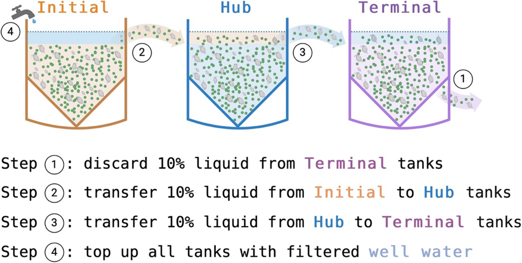
To simulate a connected landscape, we set up six replicates of a three-node unidirectional network composed of one initial node, one intermediate hub node, and one terminal node. The first serial transfer started 2 weeks after the D. magna inoculation to ensure D. magna populations had successfully colonized each tank. Twice a week thereafter, we disposed of 10% of the liquid (∼14 L) from the terminal tank and then, transferring 10% of the liquid from the initial to the intermediate hub node, and 10% of liquid from the intermediate hub to the terminal node (Fig. 1). We stirred to homogenize contents of all tanks before each transfer to ensure that we captured a representative sample of nutrients, algae, D. magna, and detrital material during each step. After completing transfers, we topped up all tanks with filtered well water to ensure all tanks maintained 140 L capacity at the end of every sampling event. To minimize contamination, each set of replicates had its own polypropylene measuring jug (Catalog #: 470328-332, Avantor, Inc.) and all shared equipment was thoroughly rinsed using filtered water between each replicate. Given that the serial transfers began at the end of week three, we only analyzed data collected after week four, resulting in 252 time series replicates (Fig. S2).

Fig. 1.

Sample collection and processing

To monitor the changes in nutrient, algal and D. magna density, we sampled each tank twice a week over 10 weeks (20 sampling events per tank, on Tuesdays and Fridays). We collected a 200 mL water sample from each tank and used a shrimp net to systematically sweep D. magna from a total volume of 5.35 L of water. We recorded water temperature and dissolved oxygen (DO) onsite using a hand-held Handy Polaris Probe (OxyGuard Internationals A/S, Denmark), and quantified algal and cyanobacterial density, D. magna density, D. magna biomass, nitrate (N), and total phosphorus concentration (P) on each sampling date.

To estimate algal density, we poured 25 mL of tank water into a glass cuvette and used the benchtop bbe PhycoProbe (bbe Moldaenke GmbH, Germany) with the bbe+++ computer software to record green and cyanobacterial density in cells mL⁻¹. We filtered 30 mL of water through a 0.45 µm Membrane Filter (Millipore Corporation, U.S.A) to remove algae and detrital material and frozen these water chemistry samples until ready for the N and total P analysis. We calorimetrically quantified nitrate using the vanadium reduction method with the Epoch microplate reader (BioTek, VT, USA, Doane and Horwáth 2003), and followed the microplate adaptation of the molybdenum blue method with persulfate digestion to estimate total phosphorus (Murphy and Riley 1962; U.S. Environmental Protection Agency 1993; Ringuet et al. 2011). All water chemistry analyses were run in quadruplicate and results below the detection limit (0.05 mg N L⁻¹ and 0.005 mg P L⁻¹) were considered 0 mg L⁻¹.

To automate the process of obtaining D. magna density and biomass, we used the “Trackdem” R package (Bruijning et al. 2018; Shaw-McDonald 2019). To obtain videos required to use this package, we first carefully poured D. magna samples into separate Petri-dishes. Then, one at a time, each Petri-dish was placed on a lightbox, which was then covered with a custom-made cardboard box with a small window where we secured a smartphone (iPhone X) to take a 15–20 s video (Shaw-McDonald 2019). This set up allowed us to take a video from a fixed distance while minimizing the amount of vibration during filming which would have otherwise interfered with particle tracking in the “Trackdem” algorithm. For samples with high D. magna density (>200 individuals/sample), we divided the sample and took multiple individually labelled videos to reduce the amount of overlapping movement. We then trimmed each video into a short 7 s segment and transformed it into 35 picture frames at 5 frames per second. These pictures were later stacked to create a still background, which allowed the “Trackdem” software to track spatial displacements of particles, their abundance, and biomass in pixels (Bruijning et al. 2018; Shaw-McDonald 2019). Since “Trackdem” assumes each particle to be a perfect circle, we calculated individual D. magna body length L (mm) from the automated output A (pixel) using a calibration curve (

L = 0.29 * \sqrt[2]{A / π} + 0.27, F_{1, 51} = 964, R^{2} = 0.95

), which was then translated into individual body mass (μg) using the formula mass = 4.341^*L^2.829 (Watkins et al. 2011; Betini et al. 2020). The number and body mass for each D. magna were then added together to create population density (count L⁻¹) and biomass (μg L⁻¹). All D. magna were returned to their tank after all the videos are taken by the end of a sampling day.

Statistical analysis and model

To account for the replication effect and the temporal variation in the time series data, we used mixed-effect models with random intercepts for Date (n = 14) and Replicate (n = 6), combined with pairwise post-hoc tests to determine the effect and the magnitude of nutrient transport on the observed densities of nutrients, detritus, green algae, cyanobacteria, and D. magna across different nodes using the following model structure:

y = N o d e + (1 | D a t e) + (1 | R e p l i c a t e)

(1)

where Node is a three-level predictor variable (initial, hub, and terminal), and y represents the suite of response variables including total phosphorus detection probability as a binomial factor (where 0 and 1 indicated a total P concentration below or above detection limit of 0.005 mg.L⁻¹, respectively), total P for samples above detection limit (mg L⁻¹), N (mg L⁻¹), DO (mg L⁻¹), green algal density (cells L⁻¹), cyanobacterial density (cells L⁻¹), D. magna density (counts L⁻¹), and D. magna biomass (μg L⁻¹). We used a mixed-effect generalized logistic regression for total phosphorus detection probabilities and calculated the mean probability (

\hat{p}

) from the estimated odds ratios z (

\hat{p} = z / 1 + z

). We specified a fixed reference level of 0 to compare changes in the mean values and provided model estimates with confidence intervals for each node position. We reported significance among initial, hub and terminal node using a pairwise post-hoc test with Holm’s correction (Kuznetsova et al. 2017; Table 1 & Table 2).

Table 1.

Table 1. The effect of serial transfer on the observed temporal variation in total phosphorus detection probability, total phosphorus concentration (mg L⁻¹), nitrate concentration (mg L⁻¹), and dissolved oxygen concentration (mg L⁻¹).

	Total P detection			P concentration			N concentration			DO concentration
Fixed effect	Odds ratios	CI	P	Estimates	CI	P	Estimates	CI	P	Estimates	CI	P
Initial node	0.08	0.01–0.60	–	0.02	0.003 – 0.03	–	0.98	0.74 – 1.22	–	10.82	8.42 – 13.22	–
Hub node	0.39	0.06–2.68	–	0.03	0.02 – 0.04	–	1.34	1.09 – 1.58	–	8.69	6.29 – 11.08	–
Terminal node	1.03	0.15–6.96	–	0.05	0.03 – 0.06	–	1.50	1.26 – 1.74	–	7.80	5.40 – 10.20	–
Post-hoc comparison	log-odds	CI	P	Estimates	CI	P	Estimates	CI	P	Estimates	CI	P
Hub—initial	1.57	0.28 – 2.87	0.009	0.01	0 – 0.02	0.037	0.36	0.23 – 0.49	< 0.001	−2.14	−2.93 – −1.34	< 0.001
Terminal—initial	2.55	1.18 – 3.92	< 0.001	0.03	0.02 – 0.04	< 0.001	0.52	0.39 – 0.65	< 0.001	−3.02	−3.81 – -2.23	< 0.001
Terminal—hub	0.98	−0.15 – 2.1	0.042	0.02	0.01 – 0.03	< 0.001	0.16	0.03 – 0.29	0.004	−0.88	−1.68 – -0.09	0.009
Random effects
Residual variance: σ²	3.29			3.44 × 10⁻⁴			0.13			4.82
Random effect variance: τ₀₀	9.47 _Sample			2.65 × 10⁻⁴_Sample			0.16 _Sample			19.95 _Sample
	0.71 _Treatment			0.95 × 10⁻⁴_Treatment			0.01 _Treatment
Interclass correlation coefficient (ICC)	0.76			0.51			0.57			0.81
	6 _Treatment			6 _Treatment			6 _Treatment
N	14 _Sample			12 _Sample			14 _Sample			14 _Sample
Observations	252			93			252			252
Marginal R²/conditional R²	0.076/0.774			0.154/0.586			0.136/0.625			0.061/0.817

Note: Statistical significance (P < 0.05) are highlighted in bold.

Table 2.

Table 2. The effect of serial transfer on the observed temporal variation in log-transformed green algal density (cells L⁻¹), cyanobacterial density (cells L⁻¹), D. magna density (counts L⁻¹), and D. magna biomass (µg L⁻¹).

	Green algal density			Cyanobacterial density			D. magna density			D. magna biomass
Predictors	Estimates	CI	P	Estimates	CI	P	Estimates	CI	P	Estimates	CI	P
Initial	16.39	16.06–16.73	–	15.48	15.19 – 15.77	–	3.28	2.82 – 3.74	–	6.20	5.82–6.59	–
Hub	16.60	16.27–16.94	–	15.58	15.29 – 15.87	–	3.62	3.16 – 4.08	–	6.48	6.10 – 6.87	–
Terminal	16.67	16.34–17.0	–	15.51	15.22 – 15.80	–	3.56	3.10 – 4.02	–	6.39	6.00 – 6.77	–
Post-hoc comparison	Estimates	CI	P	Estimates	CI	P	Estimates	CI	P	Estimates	CI	P
Hub—initial	0.21	0.08 – 0.33	< 0.001	0.1	−0.06 – 0.26	0.46	0.33	0.15 – 0.53	< 0.001	0.28	0.07 – 0.48	0.006
Terminal—initial	0.28	0.15 – 0.4	< 0.001	0.03	−0.13 – 0.20	0.67	0.28	0.09 – 0.47	< 0.001	0.18	−0.03 – 0.39	0.08
Terminal—hub	0.07	−0.06 – 0.2	0.202	−0.07	−0.23 – 0.09	0.64	−0.06	−0.24 – 0.13	0.47	−0.10	−0.31 – 0.12	0.29
Random effects
σ²	0.13			0.21			0.26			0.34
τ₀₀	0.34 _Sample			0.19 _Sample			0.72 _Sample			0.47 _Sample
	0.02 _Treatment			0.03 _Treatment			0.001 _Treatment			0.006 _Treatment
ICC	0.74			0.52			0.73			0.58
N	6 _Treatment			6 _Treatment			6 _Treatment			6 _Treatment
	14 _Sample			14 _Sample			14 _Sample			14 _Sample
Observations	252			252			252			252
marginal R² /conditional R²	0.028/0.746			0.004/0.518			0.022/0.737			0.016/0.591

Note: Statistical significance (P < 0.05) are highlighted in bold.

In addition to comparing the observed means across the network, we calculated per capita per day rates of exponential growth (

r_{i} = \frac{\log [N_{t + τ} / N_{t}]}{τ}

, where τ is the time between consecutive sampling events, either three or four days) for green algae (r₁), cyanobacteria (r₂), and D. magna (r₃) to evaluate the effect of serial transfer location (three-level factor: initial, hub and terminal), abiotic (P (mg.L⁻¹), N (mg.L⁻¹), DO (mg.L⁻¹), temperature (°C)), and biotic factors (green algae (N₁ : cells.L⁻¹), cyanobacteria (N₂ : cells.L⁻¹), D. magna density (N₃ : counts.L⁻¹), and D. magna biomass) on the rates of population change in a mix-effect linear model. Since D. magna density and D. magna biomass were highly correlated, we only used the residuals from (

\log [b i o m a s s] = 0.82 \log [d e n s i t y] + 3.5

, F_1,232= 910.4, R²= 0.8, P < 0.001) to represent D. magna biomass. We checked the collinearity of all predictor variables using variance inflation factor (GVIF^1/(2*DF)) and all variables were below the collinearity threshold of 2.5 (Johnston et al. 2018). Since this set of full models incorporated all variables (Table S1), we applied a backward elimination method to reduce non-significant effects (Chambers and Hastie 2017; Kuznetsova et al. 2017). Key factors that influenced the rate of change for green algae (r₁), cyanobacteria (r₂), and D. magna (r₃) were as follows:

\{\begin{matrix} r_{1} = a_{1} N_{1} + b_{1} N_{2} + (1 | D a t e) + c_{1} \\ r_{2} = a_{2} N_{2} + b_{2} N_{1} + (1 | D a t e) + (1 | R e p l i c a t e) + c_{2} \\ r_{3} = a_{3} N_{3} + d N_{1} + (1 | D a t e) + c_{3} \end{matrix}

(2)

where a_i and b_i represent the density-dependent intra- and inter-specific competition (a_i, b_i < 0), the intercepts c_i represent maximum per capita growth rate of species i, and d represents the positive correlation between green algae and D. magna growth rate.

To further evaluate the competitive outcome between green algae and cyanobacteria occurred in our system, we parameterized the following Lotka–Volterra competition model (Lotka 1925; Volterra 1926):

\{\begin{matrix} \frac{d N_{1}}{d t} = {r_{m a x}}_{1} N_{1} [1 - \frac{N_{1} + α_{12} N_{2}}{K_{1}}] \\ \frac{d N_{2}}{d t} = {r_{m a x}}_{2} N_{2} [1 - \frac{N_{2} + α_{21} N_{1}}{K_{2}}] \end{matrix}

(3)

where N₁ and N₂ represent green algal and cyanobacterial density, r_max₁ and r_max₂ depict their maximum growth rates (r_m_ax_i = c_i), K₁ and K₂ represent their carrying capacities (K_i = − c_i/a_i). The Lotka–Volterra competition coefficient α₁₂ indicates the per capita impact of cyanobacteria on the population growth of green algae (α₁₂ = b₁/a₁), and α₂₁ describes the impact of green algae on the population growth of cyanobacteria (α₂₁ = b₂/a₂). We used the average green algal and cyanobacterial density from sample #7 (N_{1, 0} = 5.67 × 10⁷ ; N_2,0 = 2.75 × 10⁶ cell L⁻¹) as the initial green algal and cyanobacterial density and simulated their population trajectory for 120 days and calculated the equilibrium density (where

{\hat{N}}_{1} = (K_{1} - α_{12} K_{2}) / (1 - α_{12} α_{21)})

{\hat{N}}_{2} = (K_{2} - α_{21} K_{1}) / (1 - α_{12} α_{21})

). The competitive outcome between green algae and cyanobacteria depends on both their respective carrying capacity and their competition coefficients, expressed as follows:

K_{1} > \frac{K_{2}}{α_{21}}

K_{2} > \frac{K_{1}}{α_{12}}

: two species coexist but the equilibrium is unstable;

K_{1} > \frac{K_{2}}{α_{21}}

K_{2} < \frac{K_{1}}{α_{12}}

: green algae out-competes cyanobacteria;

K_{1} < \frac{K_{2}}{α_{21}}

K_{2} > \frac{K_{1}}{α_{12}}

: cyanobacteria out-competes green algae;

K_{1} < \frac{K_{2}}{α_{21}}

K_{2} < \frac{K_{1}}{α_{12}}

: two species coexist and the equilibrium is stable.

All statistical analyses were conducted in R 2023.09.1 + 494 (R Core Team 2023). The linear mixed-effect models were fitted by maximum likelihood using the package “lme4” (Bates et al. 2015) and model coefficients were visualized using package “sjPlot” (Lüdecke 2023). Post-hoc analysis was done using the package “multcomp” and P-values were reported with Holm’s correction (Hothorn et al. 2008). Model optimization was performed using “lmerTest” package (Kuznetsova et al. 2017). All figures were created using the package “ggplot2” (Allen et al. 2019) with colour palette from “RColorBrewer” (Neuwirth 2022) and “ggtext” (Wilke and Wiernik 2022). The variance inflation factor was calculated using the package “car” (Fox and Weisberg 2019). All data and R scripts used for the analyses is made publicly available on GitHub public repository in the Data Availability Statement.

Results

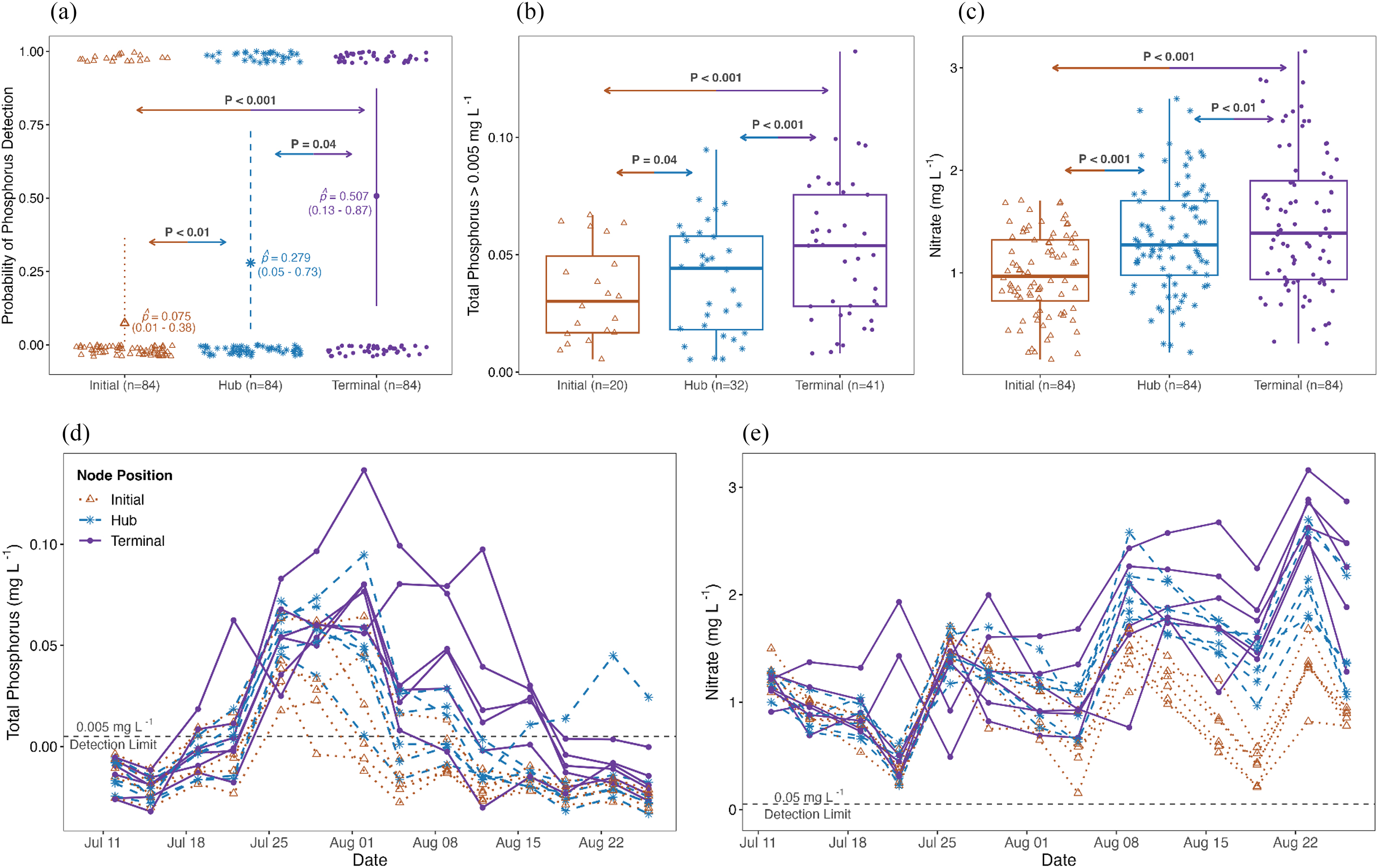
We compared the observed mean densities of nutrients, detritus load, green algae, cyanobacteria, and D. magna across the initial, hub, and terminal nodes. Nutrients showed significant evidence of downstream accumulation consistent with predictions from spatial nutrient transport theory: terminal nodes had the highest detectability and concentration of total P (p̂ = 0.51, CI = 0.13–0.87, Fig. 2a; β = 0.05, CI = 0.03–0.06, Fig. 2b; Table 1) and N on average (β = 1.50, CI = 1.26–1.74, Fig. 2c, Table 1), significantly higher than those of hub and initial nodes (P < 0.05, Table 1). We found that node position explained 15.4% and 13.6% of the variation in the observed mean total P and total N concentration (Table 1), while random effect of time and replication contributed to an additional 43% and 49% of the variation (conditional-marginal R²; Figs. 2d and 2e). This highlighted that spatiotemporal factors could contribute to as much as 62% of the observed variation in nutrient concentrations.

Fig. 2.

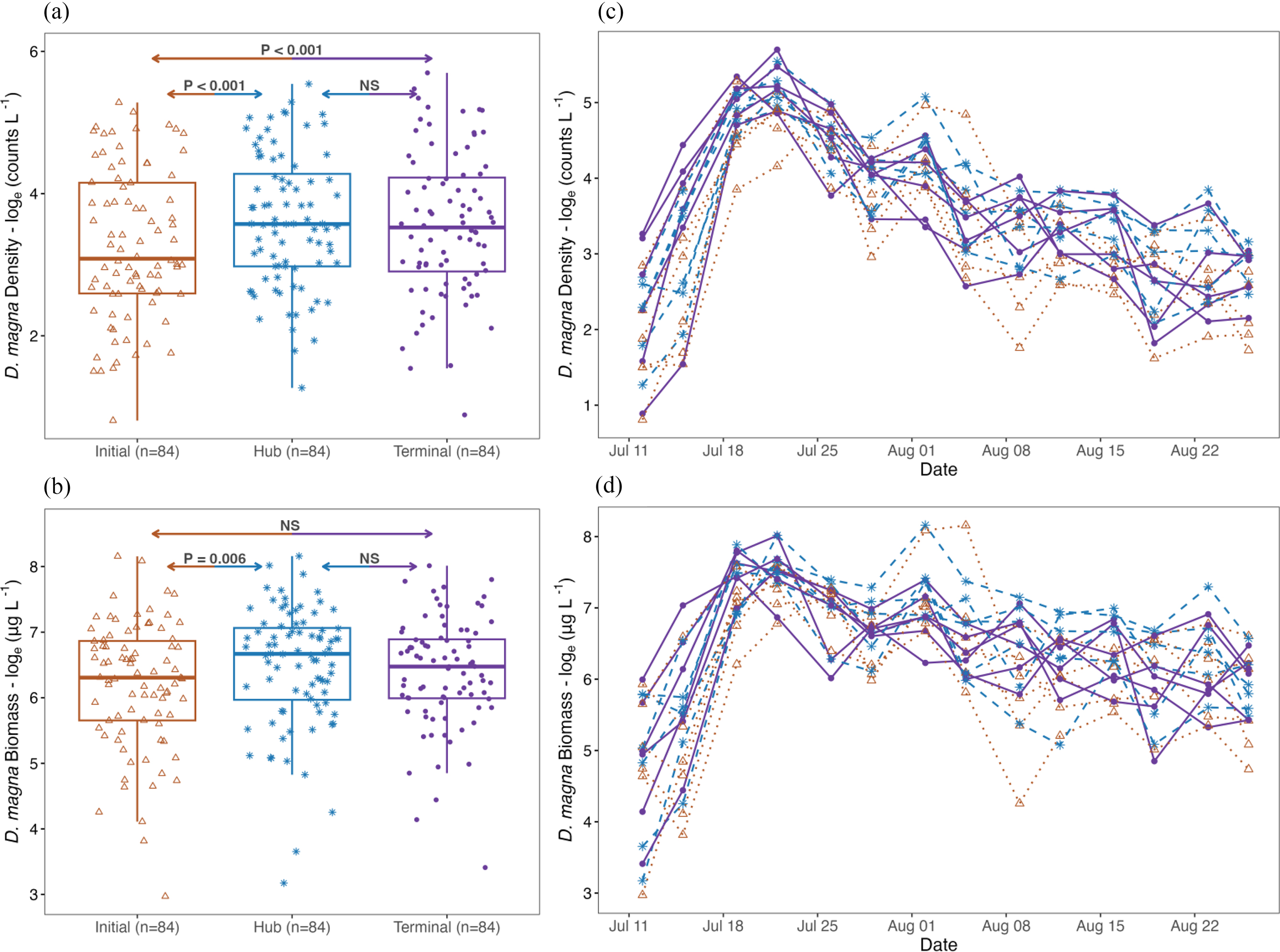
Increased levels of nutrients were associated with modest increases in the abundance of green algae and D. magna in hub and terminal nodes relative to the initial node (Figs. 3 and 4). While we found no difference between hub and terminal nodes (P > 0.05, Table 2), the initial node had the lowest densities of green algae (β = 15.48, CI = 15.19–15.77, Table 2, Fig. 3a), D. magna (β = 3.26, CI = 2.78–3.73, Table 2, Fig. 3a), and D. magna biomass (β = 7.48, CI = 7.09–7.88, Table 2, Fig. 3b). There was little evidence that cyanobacteria density responded to serial transfer, with no significant difference detected among initial, hub, or terminal nodes (P > 0.05, Table 2, Fig. 3b).

Fig. 3.

Fig. 4.

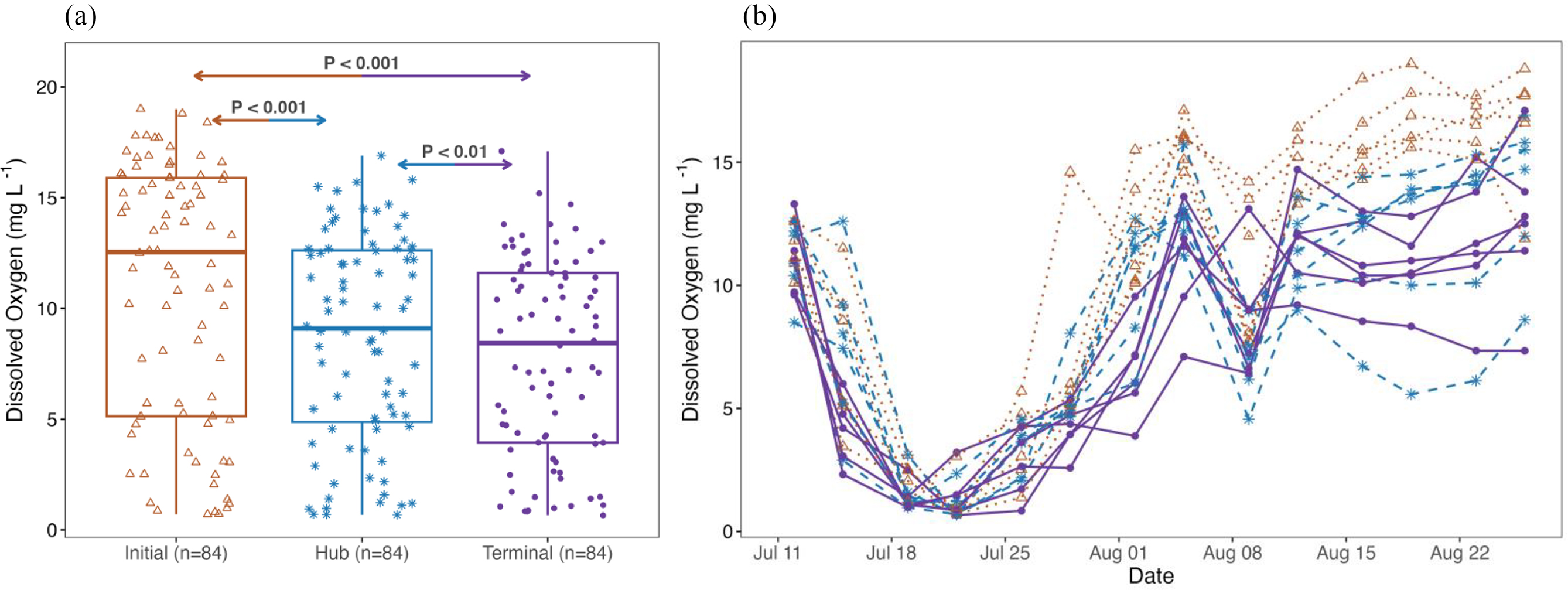
While we observed modest increase in algal and D. magna density along the spatial gradient, we found strong evidence of reduced DO concentration downstream and recorded the lowest DO concentration in the terminal nodes (β = 7.80, CI = 5.40–10.20, Table 1, Fig. 5). Given that green algae and cyanobacterial cell density, D. magna abundance, and detrital materials are all known to affect oxygen production and uptake, changes in DO concentration could be due to multiple causes. In our system where phytoplankton or zooplankton showed no difference between the hub and terminal nodes (P > 0.05, Table 2), we suggest that the decreasing DO was likely driven by increased detritus load and bacteria-driven oxygen uptake.

Fig. 5.

Tank position did not influence the exponential growth rates recorded for green algae or cyanobacteria (P > 0.05, Table S1), but exponential growth rates within tanks consistently reflected localized effects of intra- and inter-specific competition (Table 3). Green algal growth rate showed negative density dependence (a₁ = −3.00 × 10⁻⁹, CI = (−3.52 – −2.47) × 10⁻⁹, P < 0.001, Fig. 6a), and strong negative inter-specific competition with cyanobacteria (b₁ = −5.73 x10⁻⁹, CI = (−9.59 – −1.88) × 10⁻⁹, P = 0.004, Fig. 6c). Similarly, cyanobacterial growth rate decreased with cyanobacteria density (a₂ = −1.82 × 10⁻⁹, CI = (−2.48 to −1.15) × 10⁻⁹, P < 0.001, Fig. 6b) and green algae density (b₂ = −19.32 × 10⁻⁹, CI = (−24.59 to −14.1) × 10⁻⁹, P < 0.001, Fig. 6d). D. magna growth rate demonstrated strong density dependence (a₃ = −0.0023, CI = −0.003 to −0.002, P < 0.001, Table 3) and a positive response to increasing green algae abundance (b₃ = 1.15 × 10⁻⁹, CI = (0.34–1.95) × 10⁻⁹, P = 0.005, Table 3), but no apparent relationship to cyanobacteria abundance. Abiotic factors such as total P, N, DO, and temperature had no detectable influence on exponential growth rates (P > 0.05, Table S1).

Fig. 6.

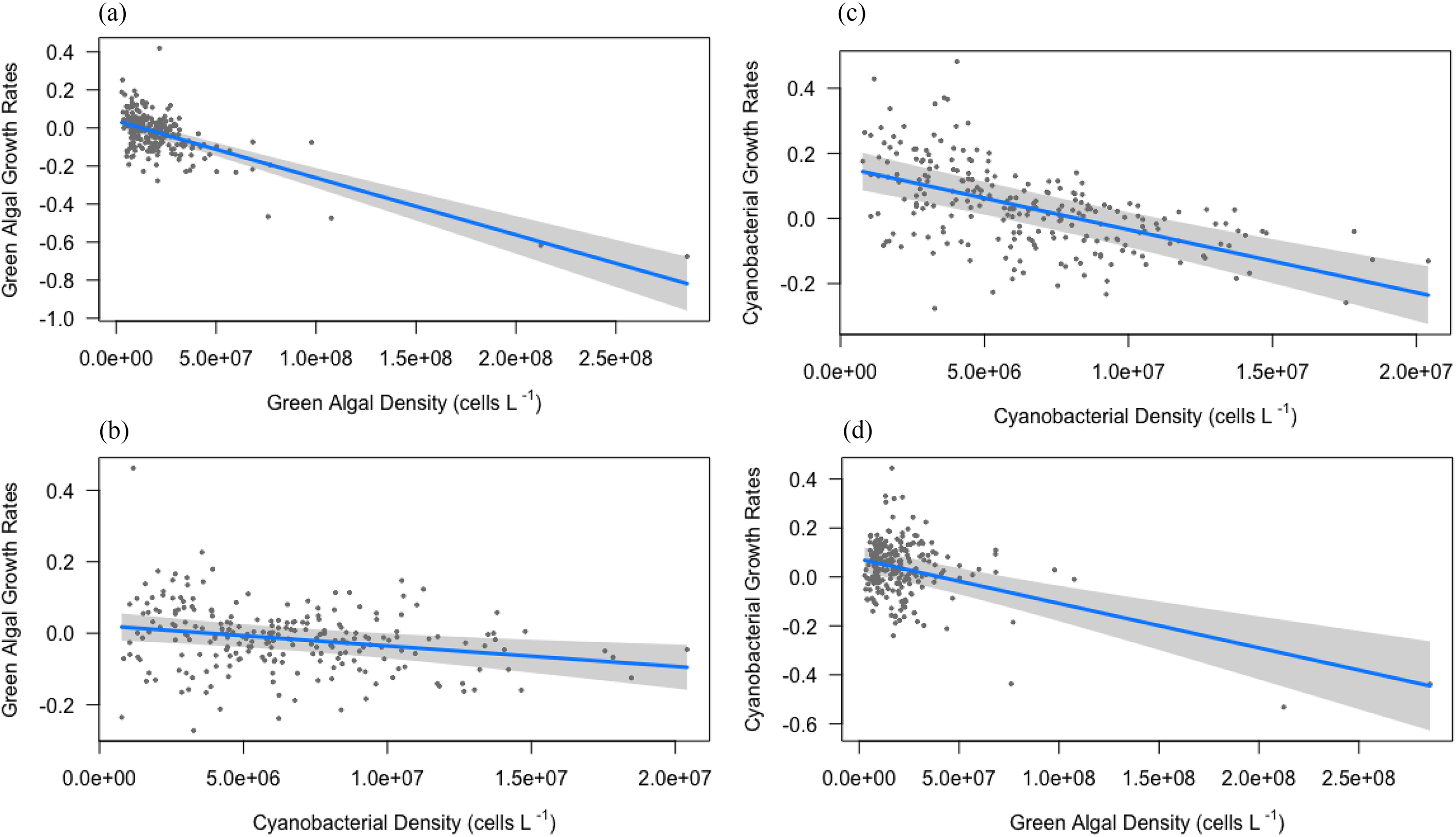
Table 3.

Table 3. The effect of green algal density (cells L⁻¹), cyanobacterial density (cells L⁻¹), and D. magna density (counts L⁻¹) on the per capita per day exponential growth rates of green algal, cyanobacterial, and D. magna density.

	Green algal growth rates			Cyanobacterial growth rates			D. magna growth rates
Predictors	Estimates	CI	p	Estimates	CI	p	Estimates	CI	P
r_max	0.071	0.03 – 0.11	0.001	0.19	0.13 – 0.25	< 0.001	0.106	0.01 – 0.21	0.051
Green algal density (cells L⁻¹)	−3.00 (×10⁻⁹)	−3.52 to −2.47 (×10⁻⁹)	< 0.001	−1.82 (×10⁻⁹)	−2.48 to −1.15 (×10⁻⁹)	< 0.001	1.15 (×10⁻⁹)	0.34 – 1.95 (×10⁻⁹)	0.005
Cyanobacterial density (cells L⁻¹)	−5.73 (×10⁻⁹)	−9.59 to −1.88 (×10⁻⁹)	0.004	−19.32 (×10⁻⁹)	−24.5 to −14.1 (×10⁻⁹)	< 0.001
D. magna density (counts L⁻¹)							−0.0023	−0.003 to –0.002	< 0.001
Random effects
σ²	0.008			0.012			0.018
τ₀₀	0.003 _Sample			0.005 _Sample			0.027 _Sample
				0.001 _Treatment
ICC	0.27			0.33			0.60
N				6 _Treatment
	13 _Sample			13 _Sample			13 _Sample
Observations	234			234			234
Marginal R² /conditional R²	0.373/0.546			0.272/0.513			0.247/0.696

Note: Regression estimates from full models can be found in Table S1. Statistical significance (P < 0.05) are highlighted in bold.

Coefficients of the Lotka–Volterra competition model suggest that even though cyanobacteria exhibited higher competitive inhibition on green algae than the converse (α₁₂ = 1.87 vs. α₂₁ = 0.094, Table 4, Fig. 7), stability analysis indicated a locally stable equilibrium with trajectories for both green algae and cyanobacteria converging on the interior intersection of their respective null isoclines (Fig. 7b).

Fig. 7.

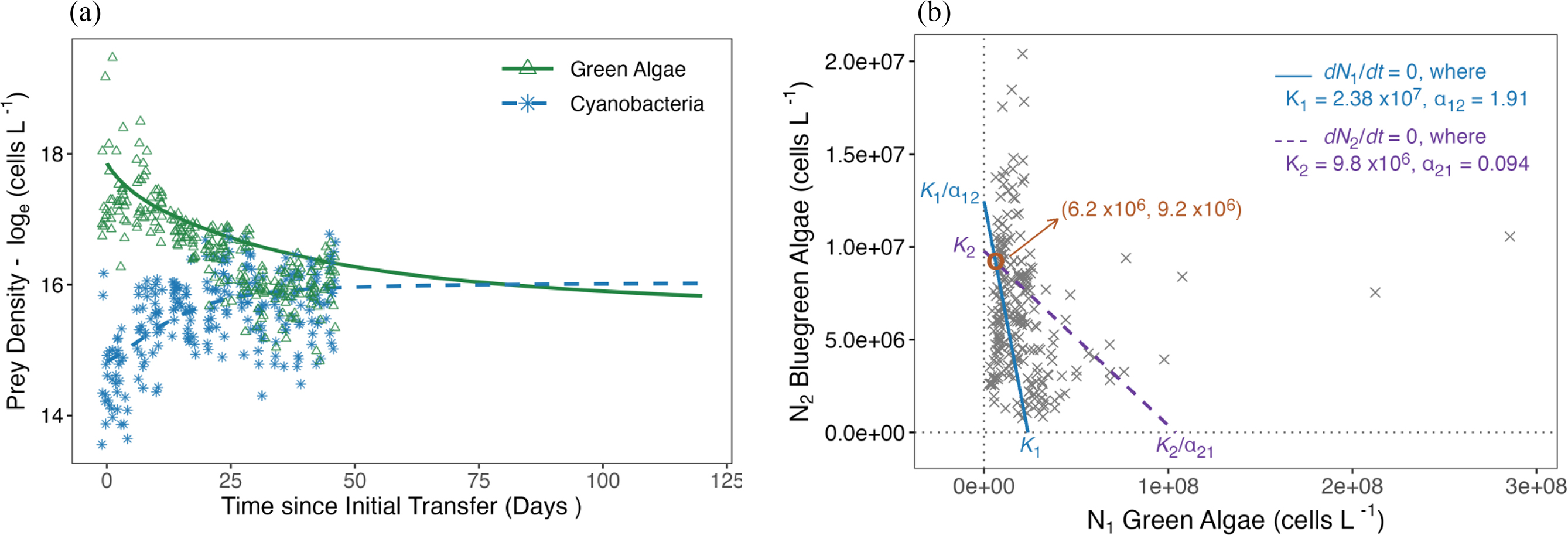
Table 4.

Table 4. Parameter values used in the Lotka–Volterra competition model to determine the competitive outcome between green algae and cyanobacteria.

Lotka–Volterra competition parameters
	Parameter	Descriptions	Value
Green algae	r_max₁	Maximum growth rate	0.071
	α₂₁	Inhibition from cyanobacteria	1.91
	K₁	Carrying capacity (cells L⁻¹)	2.38 × 10⁷
	${\hat{N}}_{1}$	Equilibrium density (cells L⁻¹)	6.2 × 10⁶
Cyanobacteria	r_t₂	Maximum growth rate	0.19
	α₁₂	Inhibition from green algae	0.094
	K₂	Carrying capacity (cells L⁻¹)	9.8 × 10⁶
	${\hat{N}}_{2}$	Equilibrium density (cells L⁻¹)	9.2 × 10⁶
Stability analysis
	K₂ = 9.8 × 10⁶ < K₁/α₁₂ = 1.24 × 10⁷
	K₁ = 2.38 × 10⁷ < K₂/α₂₁ = 1.04 × 10⁸

Discussion

From heavy usage of synthetic fertilizers and pesticide to large scale land clearing and modification, intense agricultural production is increasingly recognized as a key threat to aquatic ecosystem services (Tilman 1999; Dudley and Alexander 2017). Over half of nitrogen and phosphorus inputs from fertilizer application to farmlands can be lost to surrounding terrestrial and aquatic ecosystems, destabilizing food web structure, interrupting nutrient cycling, and reducing ecosystem functions (Bouwman et al. 2009; Zou et al. 2022). In interconnected watersheds, nutrients can travel great distances, affecting many coupled ecosystems far from the source (Loreau et al. 2003; Gounand et al. 2014; McCann et al. 2021; Tadiri et al. 2024). To test the impact of nutrient transport on the presence and magnitude of enrichment-driven instabilities across a spatial gradient, we used the classic Daphnia-phytoplankton-nutrient model system in a three-node unidirectional mesocosm experiment.

We found that even though nitrate, total phosphorus, and detrital materials accumulated significantly downstream (Figs. 2 and 5), a pattern consistent with predictions from the spatial nutrient transport theory (McCann et al. 2021), this did not result in extreme amplification of population abundance, cycling, or complete competitive exclusion of green algae in hub or terminal nodes (Figs. 3c–3d and 4c–4d). Instead, our algal/cyanobacteria community converged on a stable equilibrium, where green algae and cyanobacteria co-exist at around 6.2, and 9.2 million cells L⁻¹, respectively, independent from node position (Fig. 7b). Here, we discussed several factors at work in our system that could contribute to the stability in our system.

First, the enrichment level in our system could be inadequate. Given the detection limit of 0.005 mg P L⁻¹, we were only able to quantify total phosphorus in 37% of our total samples (n = 92), 40% of which were below the blooming threshold of 0.03 mg L⁻¹ (n = 36, Dodds et al. 2002). Even though we added liquid fertilizer weekly (∼15.8 mg P and 50 mg N Tank⁻¹), we found phosphorus uptake to be extremely rapid and that the phosphorus level sometimes dropped below the detection limit within 24 hours. Compared to the ideal 16:1 N:P ratio for algal growth, the exceedingly high stoichiometric ratio of N:P in our system (48:1 ± 43:1, n = 92) suggested that phosphorus was the limiting nutrient in our system (Guildford and Hecky 2000), which could lower algal growth rate (Li et al. 2022) and reduce the potential for complete competitive exclusion (Redfield 1934; Takamura et al. 1992; Neill 2005).

Second, strong intra- and inter-specific competition between green algae and cyanobacteria could be stabilizing. Previous work suggests that nutrient enrichment tends to amplify Daphnia-phytoplankton prey-escape cycles most readily in simple systems composed of strictly edible algal species (McCauley et al. 1999). In natural studies or experiments where less edible or unpalatable prey are present, enrichment rarely leads to prey-escape cycles (McCauley and Murdoch 1990; Murdoch et al. 1998; Genkai-Kato and Yamamura 1999; McCauley et al. 1999; Mougi and Nishimura 2007), as a result of interspecific competition among algal prey (Kretzschmar et al. 1993; Genkai-Kato and Yamamura 1999) and/or changes in predator foraging (McCauley et al. 1988, 1999; Mougi and Nishimura 2007; Yin et al. 2010). Similarly, we found that intra- and inter-specific competition between green algae and cyanobacteria were key factors influencing algal growth rates, but not D. magna abundance (P > 0.05, Table S1). Cyanobacteria had higher maximum rates of increase (r₂ = 0.19 > r₁ = 0.071, Table 4), suggesting they were more effective at nutrient uptake than green algae. Cyanobacteria exerted stronger evidence of competitive inhibition on the growth of green algae than vice versa (α₂₁ = 1.87 > α₁₂ = 0.094, Table 4). While competitive displacement by cyanobacteria did not drive green algae to complete extinction (McCann et al. 2021), it depressed long-term levels of green algal abundance to a considerable extent. Cyanobacteria reached a 50% higher density at equilibrium than green algae (9.2 × 10⁶ cells L⁻¹ vs. 6.2 × 10⁶ cells L⁻¹). This is particularly impressive in relation to the substantial difference in their respective carrying capacities (9.8 × 10⁶ cells L⁻¹ vs. 2.38 × 10⁷ cells L⁻¹).

Third, all our tanks were subject to augmented inoculations of green algae every two weeks, which could also contribute to the persistence of green algae in our system. We note that cyanobacteria slowly, and successfully, invaded our mesocosms 3 weeks after green algae density had already established population densities of 2.1 ± 1.2 × 10⁵ cells L⁻¹. It is conceivable that algal competitive outcomes might change if initial levels of abundance or temperature conditions had been different. Slow rates of cyanobacteria invasion might be expected, because per capita growth rates of M, aeruginosa are much lower at 18 °C than at 25 °C (Shaw 2020), unlike green algae C. vulgaris (Jarvis et al. 2016).

Lastly, difference in prey palatability could influence D. magna’s feeding behaviour. Our results showed that D. magna population growth rates were positively related only to green algae abundance, and there was no detectable influence of cyanobacteria abundance. This suggested that while cyanobacteria in our system are edible, they were so poorly profitable that they failed to fulfill D. magna’s energetic needs. Bench-top trials conducted in our lab were consistent with this hypothesis, showing that per capita rates of survival, reproduction, and individual mass gain by D. magna declined with an increasing ratio of M, aeruginosa to C. vulgaris in their diet (Shahmohamadloo et al. 2022). Interestingly, the lack of oscillatory predator-prey cycle from our experiment were consistent with predictions presented by Genkai-Kato and Yamamura using foraging theory (1999). In their predator-prey model, one predator could consume two prey species of varying profitability (Figs. 1a-4), and when the less palatable prey species approached the critical profitability threshold, oscillations were nearly muted. A similar theoretical prediction of behavioral stabilization comes from Fryxell and Lundberg's (1994) consumer-resource models with optimal foraging by a single consumer species and two resource species, the least profitable of which is unable to sustain predators on its own. Prey escape cycles can also be muted by resource limitation (Carroll et al. 2022; Luckinbill 1973), complexity of natural food webs (Rall et al. 2008; Kretzschmar et al. 1993; McCauley et al. 1999; Mougi and Nishimura 2007; Murdoch et al. 1998; Persson et al. 2001; Roy and Chattopadhyay 2007), landscape connectivity (Feng and Li 2015; Gounand et al. 2014; Gravel et al. 2016; Tadiri et al. 2024), behavioural plasticity (McCauley and Murdoch 1990; Mougi and Nishimura 2008), and rates of transport between interconnected ecosystems (Gounand et al. 2014; McCann et al. 2021).

There are some limitations to our study. It should be noted that our experimental design utilized a linear structure rather than a dendritic configuration (McCann et al. 2021). We recognized that linear network would likely promote instability due to the lack of asynchronous input (Anderson and Hayes 2018; Tadiri et al. 2024), and we are cautious that the enrichment level in our system might not reflect the level of enrichment in natural riverine systems. Our system has two sources of enrichment: downstream accumulation from directional movement of water, nutrient, resource, consumers, and detritus, as well as weekly enrichment of fertilizers. Future work could explore how different enrichment level may interact with landscape configurations (linear vs. dendritic) to influence meta-ecosystem stability. Additionally, sexual production of ephippia in Daphnia could influence consumer-resource dynamics (McCauley et al. 1999), and would be worth further investigation. Finally, our experiment followed a seasonal temperature regime, coupled with a constant flow rate where all nodes had the same initial conditions. In natural environment, coupled ecosystems would exhibit a higher degree of heterogeneity of varying species composition and climatic condition, which could be another important aspect for future work.

Eutrophication from agriculture runoff remains a persistent and complex problem. As nutrients rapidly travel across coupled ecosystems via increasingly interconnected landscape (Gravel et al. 2016; Loreau et al. 2003; McCann et al. 2021; Smithwick 2021), it is essential to understand the effect and magnitude of nutrient transport on food web stability. Consistent with the recent spatial nutrient transport theory (McCann et al. 2021), our Daphnia-phytoplankton-nutrient model system provided evidence of strong nutrient and detritus accumulation downstream. However, these changes did not lead to an amplified Daphnia-phytoplankton paradox cycle or complete competitive replacement of green algae by less edible cyanobacteria. Instead, our system converged on a stable coexisting equilibrium where cyanobacteria inhibited green algal growth and suppressed green algae abundance to a quarter of its normal carrying capacity. Improved stability in our system could result from nutrient limitation, prey competition and palatability, and weekly inoculation of green algae.

Acknowledgements

We thank all Aqualab staff members: Matt Cornish, Carolyn Trombley, and Mike Davies, who supported all technical aspects of this experiment. We are grateful for Matthew Pavusa and Dr. Andrew McDougall for providing training and assistance on our water chemistry analysis.

References

Alexander R.B., Smith R.A., Schwarz G.E., Boyer E.W., Nolan J.V., Brakebill J.W. 2008. Differences in phosphorus and nitrogen delivery to The Gulf of Mexico from the Mississippi River Basin. Environmental Science & Technology, 42, 822–830.

LOGIN TO YOUR ACCOUNT

Create a new account

Request Username

Change Password

Your password must have 8 characters or more and contain 3 of the following:

Password Changed Successfully

Verify Phone

Congrats!

Abstract

Introduction

Materials and methods

Experimental design

Sample collection and processing

Statistical analysis and model

Results

Discussion

Acknowledgements

References

Supplementary material

Information

Published In

History

Notes

Copyright

Data Availability Statement

Key Words

Sections

Subjects

Authors

Affiliations

Author Contributions

Competing Interests

Funding Information

Metrics

Other Metrics

Citations

Cite As

Export Citations

View options

PDF

Share

Share the article link

Share on social media