Open access

Seasonal patterns and key chemical predictors of dissolved greenhouse gases in small prairie pothole ponds

Publication: FACETS
25 June 2024

Abstract

Shallow ponds can provide ideal conditions for production of greenhouse gases (GHGs) carbon dioxide (CO2), methane (CH4), and nitrous oxide (N2O), and thus are important to include in global and regional GHG budgets. The Canadian Prairie Pothole Region contains millions of shallow natural ponds, and we investigated GHG dynamics in 145 ponds across the region. Ponds were consistently supersaturated with CH4, often supersaturated with CO2 (57% occurrence), and often undersaturated with N2O (65% occurrence). Spring measurements showed higher N2O saturation (p = 0.0037) than summer, while summer had higher CH4 (< 0.001) and CO2 (p = 0.023) saturation than spring. Ponds exhibited large physicochemical variation, yet sulfate concentration and pH were strong predictors of dissolved CH4 and CO2, respectively. No predictor was identified for N2O. The link between sulfate and CH4 has important implications as dissolved CH4 in low sulfate (<178 mg L−1) systems was much more responsive to changes in temperature. This research fills an important knowledge gap about the GHG dynamics of prairie pothole ponds and the role of water chemistry for diffuse GHG release. Our work can also be used in ongoing efforts to describe ecosystem services (or disservices) assigned to ponds in this agriculture-dominated region.

Introduction

Inland waters, including lakes, reservoirs, rivers, and ponds, are important biogeochemical processing sites in global cycles. Together, inland waters release greenhouse gases (GHGs) at scales important to include in global GHG budgets (Tranvik et al. 2009; Kirschke et al. 2013). Biogenic GHGs receiving consideration in these budgets are methane (CH4), carbon dioxide (CO2), and nitrous oxide (N2O), GHGs produced by microbes and larger organisms in the water column and in sediments via various metabolic pathways (Wetzel 2001; Schlesinger and Bernhardt 2020). GHG production varies between systems, but overall, biogeochemical cycling is often more intense in small ponds, owing to a stronger connection to the surrounding landscape (Downing 2010; Holgerson and Raymond 2016). Globally, small ponds are more common than larger systems (Downing et al. 2006); thus, ponds contribute to global GHG budgets more than their individual surface areas would suggest, leading to efforts to quantify GHG fluxes for small systems.
The Prairie Pothole Region (PPR) of North America contains millions of glacial-formed depressions called potholes that can fill with water depending on short- (intra-annual) and long-term (multi-year) moisture conditions. Seasonal variation is a fundamental characteristic of these ecosystems, especially related to hydrologic processes that affect water balance (LaBaugh et al. 1998). Ponds in this region also have highly variable water chemistry (LaBaugh 1989) and can switch between heterotrophy- and autotrophy-dominated multiple times a year (Bortolotti et al. 2016a). In many cases, pothole ponds in the PPR are under pressure from intensive agricultural land uses (clearing of wetland vegetation, nutrient runoff, and drainage) and as such, research to describe the importance of these ecosystems broadly for water security is ongoing (e.g., Spence et al. 2019).
Ponds in the region are valued in part for their potential to store carbon (C) in sediments and surrounding riparian areas (Euliss et al. 2006). Several studies have sought to describe the balance between C storage and GHG release across whole wetland basins and found that hydrology (e.g., water-filled pore space), land use, and temperature are important factors (Gleason et al. 2009; Badiou et al. 2011; Tangen, Finocchiaro, and Gleason 2015; Bansal et al. 2016). Other studies have focused on ponded zones and how GHG dynamics are related to ecosystem metabolism (Bortolotti et al. 2016a, 2019) and sediment microbiology (Dalcin Martins et al. 2017). Nonetheless, it remains difficult to assess the role of these ponds for GHG balance, as there is high variability of pond conditions in this region, and most studies have been conducted at local scales or on few sites. There is limited evidence showing how physicochemical parameters of ponds can be linked to GHG release or uptake specifically from ponded zones at regional scales, and the unique hydrology of the region contrasts that of other studies where small ponds have been studied previously. This contributes to high uncertainty in the role of wetland ponds for GHG emission that has been reported for the region (e.g., Petrescu et al. 2015).
To build on previous work and enhance understanding of dissolved GHG behaviour in natural pothole ponds, we used a survey approach spanning two seasons to investigate physicochemical controls on GHGs in ponds. Specific objectives were to (1) quantify dissolved GHG (CH4, CO2, and N2O) saturation levels and diffusive fluxes for ponds in spring and summer and (2) identify physicochemical predictors of and spring and summer GHG saturation. Given that pond area is highly dynamic within season and across years in the PPR, this study aims to clarify how physicochemical conditions and seasonality can affect the potential of ponds in the region to act as GHG sources or sinks, supporting efforts to improve wetland management in the region.

Methods

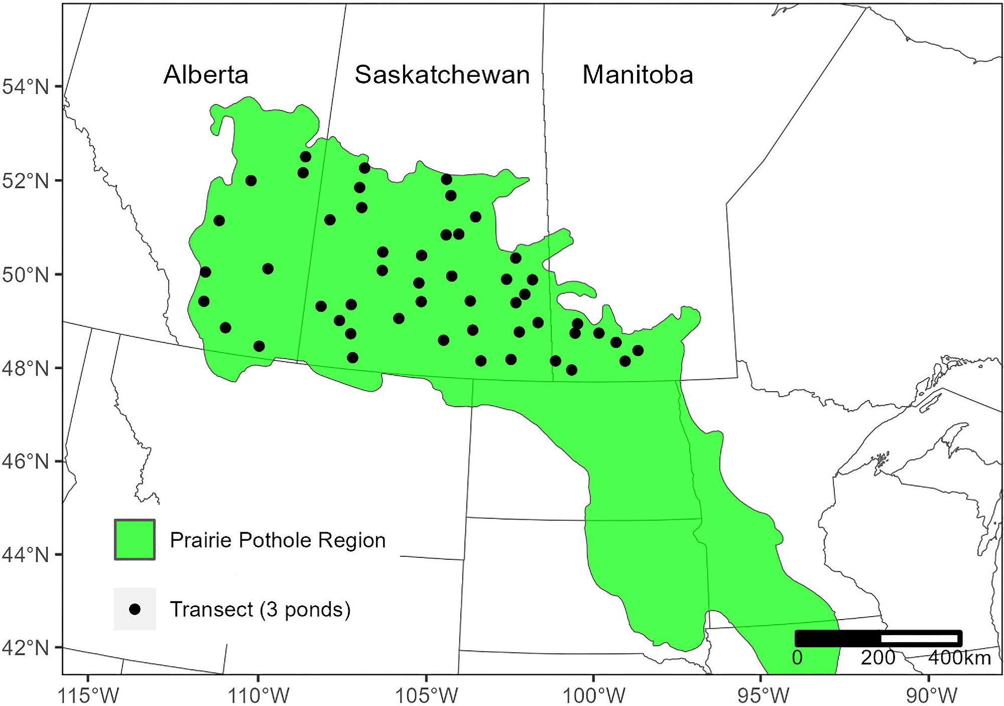
Study area and field survey

The Canadian PPR spans southern portions of the provinces of Alberta, Saskatchewan, and Manitoba where the dominant human land use is agriculture. The region has a semi-arid climate where the water balance of pothole ponds (referred to as ponds hereafter) tends to be strongly controlled by inputs from spring snowmelt and outputs from evaporation (Winter 1989; Hayashi et al. 2016). For this study, ponds were chosen from an existing database of transects used by the Canadian Wildlife Service to assess waterfowl populations via aerial and ground surveys. Fifty transects and three ponds per transect were selected for sampling (Fig. 1). The transects sampled in this study were spatially distributed across the PPR, and ponds on each transect were selected according to accessibility and likeliness to hold water through the summer. Thus, most ponds were seasonal, semi-permanent, or permanent (Stewart and Kantrud 1971) and surrounded by active agricultural land uses (crop or pasture). A team of students and technicians sampled 150 ponds in spring (26 April to 9 May 2019) and summer (23 June to 3 July 2019). Because of drier conditions in summer, which meant that some pothole depressions no longer held ponded water, only 141 ponds were sampled, 11 of which were new ponds selected from the same transect to replace a pond that had dried. Our survey approach is powerful in that it allows us to investigate a broad assemblage of physicochemical factors for their influence on GHG dynamics. The trade-off here is that it does not allow a detailed investigation of temporal changes that can occur over the growing season, which site-specific studies confer; however, because we have repeated the survey in spring shortly following snowmelt, and again in summer, our analysis of a large number of sites gives strong evidence for the regional behaviour of these systems that is not possible through local scale studies. Assessment of pond surface area was completed by McFarlan (2021) with CanVec and Canadian Wetland Inventory datasets.
Fig. 1.
Fig. 1. Map of the Prairie Pothole Region (PPR) in North America showing locations of transects (filled circles) used for this survey, with three ponds sampled per transect. Shapefiles of the PPR and North America political boundaries were obtained from the U.S. Geological Survey (https://www.sciencebase.gov/catalog).
Specific conductance (µS cm−1), pH, and water temperature (°C) were measured with a Yellow Springs Instruments (YSI) sonde at ∼20 cm depth. When no YSI sonde was available, water temperature was measured via thermometer and specific conductance and pH were measured in the Roy Romanow Provincial Laboratory (RRPL) within 72 h of sampling. We compared field- and lab-measured pH for sites where both were measured, with lab-measured pH only slightly higher than field values. We used the median difference (0.18) to correct lab-measured pH to provide a more consistent metric across all sites. Note that our results are not sensitive to use of two pH measurement methods; we tested this and found that the patterns reported below were consistent when the data were re-analysed without sites for which only lab pH was available. Atmospheric pressure (hPa) and wind speed (m s−1) were collected in the field via hand-held sensors (Kestrel Instruments, Boothwyn, United States).
Bulk water samples were collected ∼10 cm below the surface in acid-washed 1 L HDPE bottles rinsed with site water. Site water was preserved by filtering and acidifying according to the analyte (Supplementary Table S1) and stored at ∼4 °C for transport to the laboratory. Water samples for isotopic analysis were collected in separate glass containers that were filled and capped underwater to prevent any headspace. In the spring survey, sediment samples were collected at 140 ponds from water depths >30 cm using polycarbonate tubes and stored at ∼4 °C. No sediment samples were collected in summer because we assumed there would be little change in sediment characteristics between surveys. Qualitative descriptions of each pond were also recorded, including permanence classification according to Stewart and Kantrud (1971), vegetation (presence/absence of select species surrounding the pond), and adjacent land use.
Gas samples to quantify dissolved GHG concentrations in ponds were collected using headspace equilibration following Whitfield et al. (2011). A 1.1 L glass bottle was filled with site water 10 cm below the surface, which restricted sampling to ponds with sufficient water depth (≥20 cm). The bottle was quickly sealed with a silicone stopper to ensure no headspace remained. Two valves connected to the stopper were used to introduce a headspace by attaching polypropylene syringes to remove 60 mL of water and simultaneously replace it with 60 mL of ambient air. The bottle was shaken for 2 minutes in the shade to equilibrate dissolved gases in the water with the headspace air. After shaking, replicate 20 mL headspace gas samples were removed and forced into evacuated 6 mL glass Exetainer® vials. A reference ambient air sample was also collected on site, and as with ambient air used to create headspace, this was collected away from potential contamination (e.g., upwind of sampling activity).

Laboratory analysis

A discrete wet chemistry analyser (SmartChem170, WESTCO Scientific Instruments Inc., Milford, United States) was used to measure concentrations of sulfate (SO42−), total phosphorus (TP), total dissolved phosphorus (TDP), soluble reactive phosphorus (SRP), total nitrogen (TN), total ammonia nitrogen (TAN), total oxidised nitrogen (NOx: nitrate (NO3) + nitrite (NO2)), and urea (Supplementary Table S1). Alkalinity, measured as calcium carbonate (CaCO3), was also analysed on the SmartChem 170. Dissolved organic carbon (DOC) was measured in duplicate on an Aurora 1030 TOC analyser (OI Analytical) after filtration (0.45 µm). Water samples for chlorophyll a (chl a) were filtered through a glass microfiber filter (GF/F), with filters stored frozen. Filter residue was extracted with ethanol and centrifugation and analysed in cuvettes by spectrometry at 665 nm (corrected for turbidity and chlorophyll b at 750 and 649 nm, respectively), using a UV 1601 PC UV-Visible Spectrophotometer (Shimadzu Scientific Instruments, Columbia, United States).
Stable hydrogen (H) and oxygen (O) isotope ratios of water were analysed for a subset of samples (n = 48) using Los Gatos Research liquid and vapor water off-axis integrated-cavity output spectroscopy machines (ABB Inc., Quebec City, Canada). Isotope ratios report sample 18O/16O (δ18O) and 2H/1H (δ2H) values compared to Vienna Standard Mean Ocean Water-Standard Light Antarctic Precipitation (VSMOW-SLAP) according to international standards (Coplen 1996). We also calculated deuterium excess (d-excess) of water (defined as d-excess = δ2H – 8 x δ18O; Dansgaard 1964). Deuterium excess is commonly used as an indicator of the effect of evaporation on δ2H (Gibson et al. 2005; Jasechko 2019; St Amour et al. 2005; Whitfield et al. 2011; Pfahl and Sodemann 2014). In surface waters where non-equilibrium evaporation occurs, 2H tends to be depleted compared to 18O due to the slower movement of water isotopologues containing 18O.
Additionally, water samples from study sites in Saskatchewan were sent to the RRPL for additional water chemistry analyses, including dissolved ions. Magnesium, potassium, sodium, and calcium were measured via inductively coupled plasma mass spectrometry (ICP-MS); bicarbonate and carbonate were calculated from alkalinity; and chloride, fluoride, and sulfate were measured via ion chromatography. Ion concentrations were used to approximate salinity of the samples.
Sediment samples were analysed for particle size and carbon content—total, organic, or inorganic measured as % weight—and methods are described in detail by McFarlan (2021). Briefly, total carbon (TC) and OC samples were ground to a fine powder with a ball mill and ignited at 1350 °C in a nickel-lined ceramic boat (C632 C analyser, LECO, Mississauga, Canada). Prior to ignition, OC samples received multiple sulfuric acid (H2SO4) treatments until reactions stopped. The inorganic carbon (IC) fraction was determined as the difference between TC and OC. For particle size analysis, sediment samples were combusted at 400 °C for 16 h and then analysed in triplicate via laser ablation (Particle Size Analyser LA-950V2, HORIBA Canada Inc., London, Canada). Sediment size fractions of clay, silt, and sand were determined by averaging the triplicate measurements (McFarlan 2021).
Gas samples were analysed with a gas chromatograph (456-GC, Scion Instruments, Goes, The Netherlands) using a Combi PAL autosampler (CTC Analytics AG, Zwingen, Switzerland). A flame ionization detector (FID) was used to quantify CH4 <100 000 ppmv, while a thermal conductivity detector (TCD) was used for CH4 >100 000 ppmv and CO2, and an electron capture detector (ECD) for N2O. Gas standards were run at the beginning of each GC run and every 50 samples to check the GC performance and calibrate N2O (CO2 and CH4 used calibrations developed for longer-term use).

GHG calculations

For quality assurance, GHG data were screened based on % difference of the replicates before analysis. The upper limit for acceptable % difference depended on the mean replicate concentration (Supplementary Table S2) because using the same % difference for all samples tended to reject a disproportionate number of samples with low concentrations. Human error, such as improper transfer of gas from collection bottle to the Exetainers® in the field or failure to accurately transcribe Exetainer® numbers, or faulty Exetainer® seals are likely to have resulted in differences between replicates high enough to require their exclusion. After screening, the mean % difference for headspace equilibration replicates was 4% for CH4, 5% for CO2, and 2% for N2O.
Dissolved GHG concentrations (mol L−1) in the pond at the time of sampling (Cdiss) were calculated as follows:
Cdiss= (nhs-namb+nwater) Vwater
(1)
where nhs is moles of gas in the headspace post-equilibrium, namb is the moles of gas from ambient air in the headspace, nwater is moles of gas dissolved in the water post-equilibrium, and Vwater is the volume (L) of water. Headspace and ambient air GHG data (ppmv), site temperature, local pressure, and headspace volume were used with the ideal gas law to find nhs and namb. According to Henry’s Law, nwater is related to nhs by a solubility coefficient, and the coefficient can be expressed as a function of temperature and salinity. For CO2 and N2O, the coefficient F (mol L−1 atm−1, eq. 2) was used (Weiss and Price 1980) and for CH4 the coefficient β (L gas dissolved in 1 L of water, eq. 3) was used (Yamamoto et al. 1976).
lnF=A1+A2100T+A3lnT100+A4T1002+SB1+B2T100+B3T1002
(2)
lnβ=A1+A2100T+A3lnT100+SB1+B2T100+B3T1002
(3)
The constants A1–A4 and B1–B3 are specific to each gas and equation, T is water temperature (K) measured at the time of sampling and S is salinity (‰). For sites without major ion concentration data, salinity was approximated from specific conductance using a regression equation developed using the Saskatchewan sites. Using the coefficients F and β, we calculated nwater by the separate equations:
nwater=xhs×F×Vwater
(4)
nwater=βPCH4VwaterR×273.15
(5)
where R is the universal gas constant. Molar fraction (xhs) for CO2 and N2O and partial pressure (in atm) for CH4 (PCH4) were used. Saturated GHG concentrations (Csat), when pond water is in equilibrium with the atmosphere, were also calculated but using seasonal mean (spring or summer) ambient concentrations of CH4, CO2, and N2O (xamb) instead of headspace concentrations.
We then calculated difference between observed dissolved GHG concentrations and equilibrium concentrations (ΔGHG) (mol L−1), the difference between Cdiss and Csat, such that negative values represent undersaturation. Delta GHG concentrations show the magnitude by which pond water is oversaturated or undersaturated. Percent saturation of dissolved GHGs in water (%GHG) was also calculated to categorise ponds as undersaturated (<95%GHG), saturated (≥95 and ≤ 105%GHG), or supersaturated (>105%GHG) and was used instead of ΔGHG for some analyses where negative values could not be used.
For observations that were undersaturated or supersaturated, GHG fluxes (FluxGHG) were calculated by multiplying gas transfer velocity, k (cm h−1), by ΔGHG (eq. 6). Then GHG fluxes were converted to mmol m−2 d−1 for CO2 or CH4 and µmol m−2 d−1 for N2O. We approximated k using two different wind models, a model based on a small lake in New Hampshire (eq. 7; Cole and Caraco 1998) and another established for wetland ponds in Florida (eq. 8; Sebacher et al. 1983). Sebacher et al. (1983) describe their model (eq. 8) applying to windspeeds between 1.4 and 3.5 m s−1, measured at 2 cm, but we applied it to the full range of windspeeds observed.
FluxGHG=kGHG×ΔGHG
(6)
kGHG,Cole=2.07+0.215×U101.7×ScGHG600n
(7)
kGHG,Sebacher=1.1+1.2×U0.021.96×ScGHGScCH4,20°Cn
(8)
Wind speed measured at 2 m in the field was converted to wind speed at 10 m (U10) or 0.02 m (U0.02) using the power-law wind profile and assuming neutral stability conditions (Arya 2001). The Schmidt number, Sc, refers to the diffusive properties specific to each GHG and was calculated, correcting for the effect of temperature by the equation, from Wanninkhof (1992):
Sc=A-BT+CT2-DT3
(9)
where AD are gas-specific constants obtained from Wanninkhof (1992) who summarised the original work of Jähne et al. (1987) and Wilke and Chang (1955). The ratio of Schmidt numbers was used to adjust k for the correct gas and temperature, and the exponent n of –2/3 for smooth surface conditions (Jähne et al. 1987) was used. A smooth surface was likely because the ponds have small surface area, shallow depth, and perimeter vegetation, all of which limit wave formation.
Lastly, we calculated CO2 equivalents (CO2-eq) to compare how fluxes of each GHG contribute to the radiative balance of the global energy budget (Neubauer 2021). Methane and N2O fluxes (as g m−2 d−1) were multiplied by the global warming potential (GWP; Table 7.15 in Forster et al. 2021) for both 20- and 100-year time horizons (CH4: GWP20 = 79.7 and GWP100 = 27.0; N2O: GWP100 = 273, and GWP20 = 273). We treated our GHG fluxes as one-time pulses because our data collection did not allow for a robust estimation of season-long GHG fluxes.

Statistical analysis

All calculations and analyses were performed in R (R Core Team 2023) and results were visualised using R packages ggplot2 (Wickham 2016), ggforce (Lin Pedersen 2022), and cowplot (Wilke 2020). To explore relationships between GHGs, water, and sediment properties, we used principal components analysis (PCA). Highly skewed variables were identified by Shapiro–Wilk test (R Core Team 2023, function: shapiro.test) and square root transformed to reduce the effect of extreme values. All variables were scaled to unit variance for PCA analysis (R Core Team 2023, function: prcomp). Resulting variable scores were scaled proportional to the eigenvalues so that angles between variables in the PCA biplot (Fig. 2) show correlation. Input variables (n = 17) were constrained to those with few missing observations, as missing values are problematic for PCA.
Fig. 2.
Fig. 2. Correlation biplotshowing results from principal component analysis examining greenhouse gas saturation and physicochemical variables for spring and summer ponds. Points are individual observations plotted according to their values along the new axes, principal component (PC) 1 and PC2, which explained 23% and 16% of the variation, respectively. 61% of the variation in the data are not shown. Lines represent the loading of labeled variables and angles between variables show correlation. Variables that were highly skewed (%CH4, %CO2, %N2O, ChlA, specific conductance, SO42–, NOx, and TAN) were square root transformed and all variables were scaled to unit variance (mean = 0 and standard deviation = 1) prior to this analysis. Note: Variable abbreviations are as follows: %CH4, methane saturation; %CO2, carbon dioxide saturation; %N2O, nitrous oxide saturation; ChlA, chlorophyll a; DOC, dissolved organic carbon; NOx, total oxidised nitrogen (NO3, nitrate +  NO2, nitrite); Sed TC; sediment total carbon; Sp. Cond., specific conductance; Temp, water temperature; TAN, total ammonia nitrogen; TDP, total dissolved phosphorus; TP, total phosphorus; TN, total nitrogen.
Relationships between GHGs and physicochemical variables were assessed using a correlation matrix approach (Harrell 2023; function: rcorr), followed by linear regression. Spearman rank correlation was used because most variables had positively skewed distributions. The false discovery rate (FDR) method was used to adjust p-values (Jafari and Ansari-Pour 2019). Where Spearman rank correlation coefficients were significant, a threshold rho > |0.25| was used to identify relationships that would be investigated via linear regression. For linear regression models, we pooled data across seasons, assessed the scatterplot of each univariate relationship, chose variable transformations (e.g., square-root and logarithm) or polynomial equations based on a priori relationships, and fit the model (R Core Team 2023, function: lm). Models were evaluated based on the adjusted R2 and FDR-adjusted p-values. To compliment linear regression, we used generalized least squares (GLS) regression (Pinheiro et al. 2021, function: gls), allowing us to investigate season as a fixed effect. We used an exponential or power variance structure on the fitted values from a global linear model to address heteroskedasticity in the data. As above, candidate variables identified by rho values were included in the model for each GHG and collinear variables were removed until all variables had a variance inflation factor below 3 (Fox and Weisberg 2019, function: VIF). Then variables were removed one by one and compared with Akaike's Information Coefficient (AIC; R Core Team 2023, function: AIC) where the model with the lowest AIC was considered the top model.
To compare spring and summer conditions for GHG and explanatory variables, we used paired t-tests (parametric) and Wilcoxon’s signed-rank tests (non-parametric). We included only the ponds that were sampled at both time points (n = 123). The paired t-test was used if differences between pairs were normally distributed for a variable (McDonald 2014), otherwise the signed-rank test was used (R Core Team 2023, functions: t.test, wilcox.test). FDR-adjusted p-values were used to identify significant differences between seasons. Direction of change between seasons was determined by the mean or median of the differences.

Results

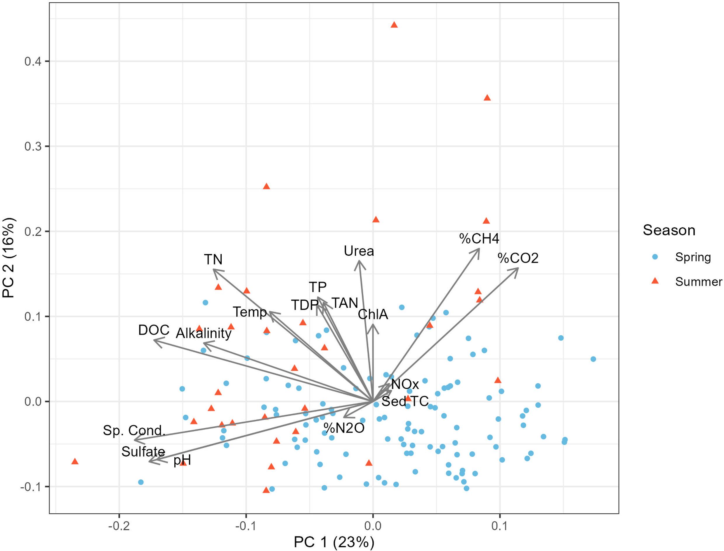
Pond physicochemical conditions

In this analysis, only ponds with sufficient water depth for GHG sampling were included, totalling 145 ponds in spring and 135 ponds in summer. Ponds were classified (Stewart and Kantrud 1971) as temporary (3%), seasonal (39%), seasonal/semi-permanent (4%), semi-permanent (41%), or permanent (13%). Ponds were small, with a median surface area of 1000 m2 or 0.001 km2. Few ponds (5%) appeared to be physically modified by humans. Overall, study ponds exhibited highly variable physicochemical conditions (Table 1), ranging from fresh to brackish, with most ponds being alkaline (median alkalinity of 200 mg L−1) with pH ≥ 7.5. DOC ranged from 10 to 140 mg L−1. Concentrations of TP, TN, and chl a indicate that most ponds were eutrophic. Pond sediments were dominated by fine particles; on average, sediments were 4% clay, 65% silt, and 31% sand. Sediment C was predominantly in organic form; only 27% of sediment samples contained a small amount of measurable inorganic C (subset range: 0.02%–2.4%). Mean water temperature was 8.4 °C in spring and 20.4 °C in summer.
Table 1.
Table 1. A summary of physicochemical parameters and ΔGHG concentrations measured for pothole ponds in 2019.
ParameternUnitMin.MeanMedianMax.
Alkalinity275mg L−128250200760
Chl aµµg L–10177.0210
Cond.256µS cm−19012007707300
pH255 6.77.88.211
DOC259mg L−19.83330140
SO42−277mg L−17.04601505500
TP276mg L−10.0180.740.464.4
TDP277mg L−10.0060.60.344.4
SRP211mg L−10.00280.510.284.4
TN274mg L−10.2632.622
Urea278mg L−10.010.0810.061.3
TAN276mg L−10.00360.0490.0161.9
NOx258mg L−10.0580.240.210.89
Sediment TC122% weight1.58.36.729a
Sediment IC116% weight00.1602.4
Sediment OC117% weight1.78.97.130a
Sediment clay119%1.63.73.58.4
Sediment silt119%34666587
Sediment sand119%8.5313162
Surface area194m2282600100019 000
Twater279°C1.6141431
Wind speed242m s−102.01.86.2
δ2H48−200−130−140−58
δ18O48−24−15−15−0.88
d-excess48−51−15−155.1
ΔCH4246µmol L−10.00704.00.72120
ΔCO2242µmol L−1−26878.41100
ΔN2O261µmol L−1−0.0100.00056−0.00130.24

Note: Parameters are alkalinity, chlorophyll a (chl a), specific conductance (Cond.), pH, dissolved organic carbon (DOC), sulfate (SO42), total phosphorus (TP), total dissolved phosphorus (TDP), soluble reactive phosphorus (SRP), urea, total ammonia nitrogen (TAN), total oxidised nitrogen (NO x: nitrate (NO3 ) + nitrite (NO2 )), sediment total carbon (TC), inorganic carbon (IC), organic carbon (OC), clay, silt and sand, water temperature ( Twater), hydrogen and oxygen isotope ratios (δ2H and δ18O), and deuterium-excess (d-excess). ΔGHG concentrations are the difference between dissolved concentrations and theoretical conditions under equilibrium with the atmosphere for methane (CH4), carbon dioxide (CO2), and nitrous oxide (N2O).

a
Note that different methods for TC and OC analysis can result in small differences in maximums for these values.

Pond GHGs

Across all pond observations, CH4 was always supersaturated, while CO2 was supersaturated for 57% of measurements and N2O was undersaturated in 63% of measurements (Table 2). The distribution of GHG saturation was highly positively skewed. Because of extreme or outlier values, we use the median to represent GHG data. Median ΔGHG concentrations were 0.72 µmol L−1 ΔCH4, 8.4 µmol L−1 ΔCO2, and –0.0013 µmol L−1 ΔN2O (Table 1). Ponds undersaturated in CO2 had a median ΔCO2 of –11 µmol L−1 and supersaturated ponds had a median ΔCO2 of 58 µmol L−1. Ponds undersaturated in N2O had a median ΔN2O of –0.002 µmol L−1 and supersaturated ponds had a median ΔN2O of 0.003 µmol L−1.
Table 2.
Table 2. The proportion (%) of pond observations that were supersaturated, saturated, or undersaturated with GHGs compared to the atmosphere in spring and summer.
GHGSeasonnaSupersaturated (%)Saturated (%)Undersaturated (%)
CH4Spring14010000
 Summer10710000
CO2Spring13563.03.034.0
 Summer10851.82.845.4
N2OSpring14418.022.959.0
 Summer11814.414.471.2
a
Number of observations less than total number of ponds sampled due to exclusion of samples through screening steps. Ponds with %GHG ≥ 95 and ≤ 105 are classified as saturated to account for uncertainty.

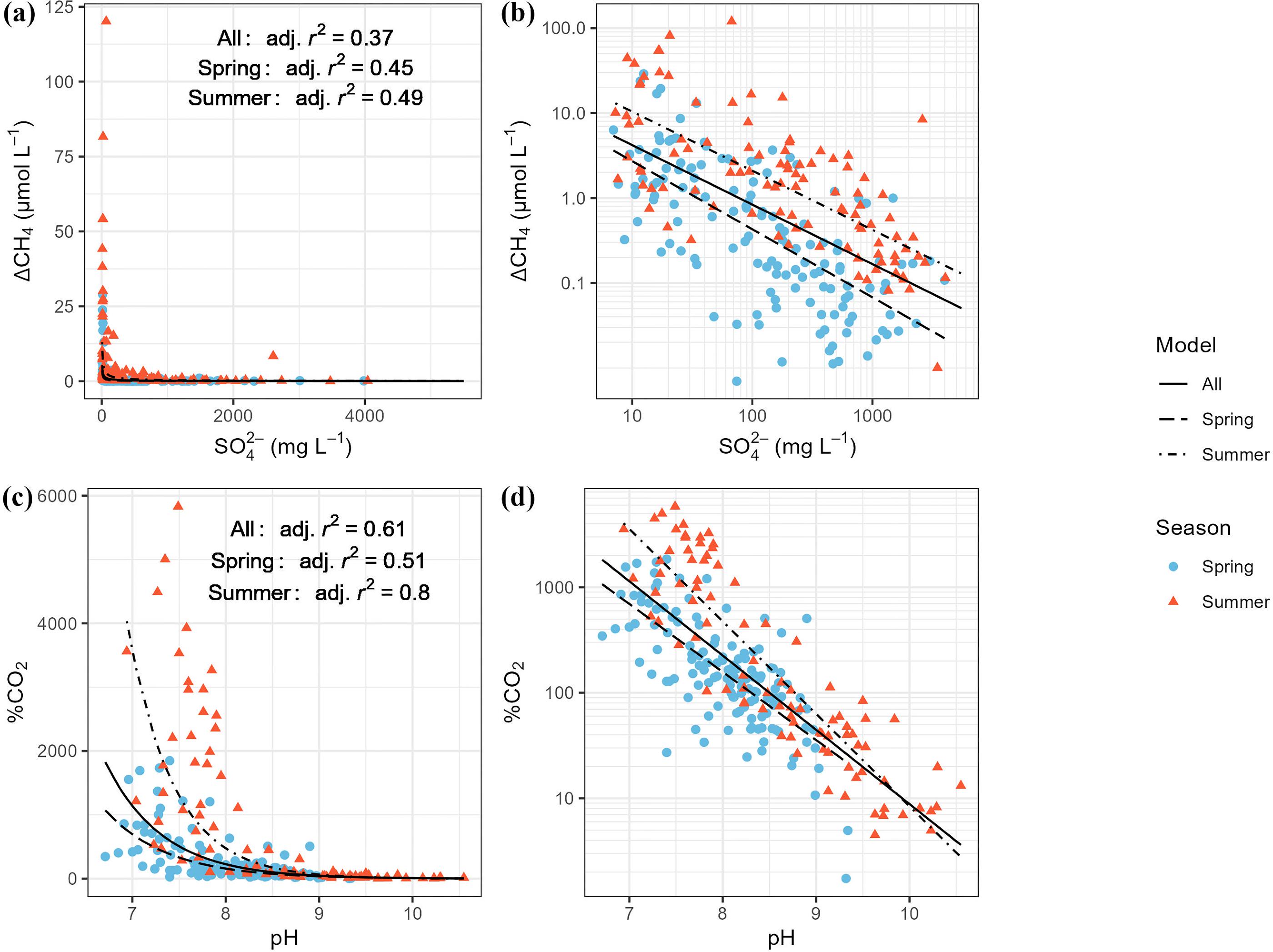
Physicochemical predictors of GHGs

Principal components (PC) 1 and 2 explained 23% and 16% of the variation in the data and had eigenvalues of 3.87 and 2.80, respectively (Fig. 2). Alkalinity and DOC had a high degree of correlation with one another and load strongly on PC1. Specific conductance, pH, SO42–, DOC, and alkalinity had the highest loadings on PC1 and so may drive the first level of variation in the dataset. Both %CO2 and %CH4 were strongly loaded on PC2 (Supplementary Table S3) and were positively correlated with each other and negatively correlated with pH, SO42–, and specific conductance (Fig. 2). Urea and TN were also strongly loaded on PC2. Fig. 2 does not show PC3 (13% variation explained), but variables %N2O, NOx, TAN, TDP, TP, and temperature were strongly loaded on this component (Supplementary Table S3).
Spearman rank correlation coefficients (Table 3) show that the physicochemical variable most strongly correlated with ΔCH4 was SO42− and with ΔCO2 and ΔN2O was pH. Pond pH was correlated with each ΔGHG but most strongly with ΔCO2. Weaker but significant relationships included ΔCH4 and water temperature, urea, and chl a; ΔCO2 and SO42–, specific conductance, and urea; and ΔN2O and SO42−. Many physicochemical variables were strongly correlated with each other but were not related to ΔGHGs (Supplementary Table S4). Notably, DOC and sediment TC were not correlated with ΔCH4 or ΔCO2. Results were similar whether ΔGHG or %GHG values were used in this analysis.
Table 3.
Table 3. Relationships between ΔGHGs and physicochemical variables were assessed by Spearman rank correlation and coefficients reported with significance level (p-values FDR-adjusted).
 %CH4%CO2%N2O
ΔCH41.0**0.51**−0.56**
ΔCO20.51**0.99**−0.44**
ΔN2O−0.53**−0.45**0.98**
Alkalinity−0.01−0.03−0.08
Chl a0.19**0.06−0.04
Cond.−0.48**−0.33**0.17*
DOC0.0−0.21**−0.08
NOx0.14*0.14*0.02
pH−0.32**−0.8**0.28**
Sed TC−0.060.17*−0.05
SO42−−0.59**−0.39**0.29**
TAN0.2**−0.03−0.1
TDP0.070.1−0.01
TP0.130.11−0.05
TN0.1−0.18*−0.05
Urea0.22**0.24**−0.15*
Twater0.32**−0.09−0.17*
**
p < 0.01
*
p < 0.05

Note: Correlations between physicochemical variables were analysed, but coefficients were not included here (Supplementary Table S4). Variable abbreviations are as follows: CH4, methane; CO2, carbon dioxide; N2O, nitrous oxide saturation (i.e., the difference between observed and theoretical equilibrium conditions) as % (%) and delta values (Δ); Chl a, chlorophyll a; Cond, specific conductance; DOC, dissolved organic carbon; NOx, total oxidised nitrogen (NO3−, nitrate +  NO2−, nitrite); Sed TC, sediment total carbon; SO42−, sulfate; TAN, total ammonia nitrogen; TDP, total dissolved phosphorus; TP, total phosphorus; TN, total nitrogen; Twater, water temperature.

Results from linear regression model fitting demonstrated that moderate amounts of the variability in ΔCH4 and %CO2 can be explained by SO42− and pH, respectively (Table 4; Fig. 3). Models of %N2O with pH and SO42− had low adjusted R2. While high values (defined here as values greater than the 75th quantile plus 1.5 times the interquartile range) for ΔCH4 occurred over a relatively narrow range of observed SO42− concentrations (6.98–178 mg L−1), highly supersaturated CO2 conditions occurred over a third of the pH range (6.9–8.1). While these models provide evidence of the broad patterns in CH4 and CO2 saturation levels, the adjusted R2 values were still low to moderate and there is considerable variability associated with these relationships, especially across seasons.
Fig. 3.
Fig. 3. Plots of the key physicochemical variable for CH4 and CO2 saturation. The top row shows ΔCH4 and sulfate (SO42−) concentration with power relationships modelled for spring, summer, and all observations (raw (a) and log-transformed (b)). The bottom row shows %CO2 and pH with exponential relationships modelled for spring, summer, and all observations (raw (c) and log-transformed (d)). Point colour and shape distinguish between seasons.
Table 4.
Table 4. Results from linear regressions to describe physicochemical predictors for GHG saturation levels in pothole ponds.
Variable pairFunctionAdjusted R2p-value
ΔCH4–SO42−Power0.36<0.001
ΔCH4–pH2nd order polynomial0.17<0.001
ΔCH4–TwaterExponential0.07<0.001
%CO2–pHExponential0.61<0.001
%CO2–SO42−Power0.14<0.001
%CO2–UreaLinear0.14<0.001
%N2O–pHExponential0.05<0.001
%N2O–SO42−Power0.06<0.001

Note: ΔGHG data were used for CH4, otherwise %GHG data were used to avoid negative values. For each variable pair, we tested different functions to describe the relationship. Displayed in this table is the model for each pair with the highest adjusted R2 that had significant p-values for the coefficients. Variable abbreviations are as follows: ΔCH4, methane saturation; %CO2, carbon dioxide saturation; %N2O, nitrous oxide saturation; SO42−, sulfate; Twater, water temperature.

GLS regression identified that season was a significant factor for both CH4 and CO2, but not for N2O. The top GLS model for CH4 included SO42–, pH, and season and all parameters were significant (p ≤ 0.01) and well estimated (Supplementary Table S5). Water temperature was collinear with season, so only season was used in the ΔCH4 model. Delta CH4 decreases as both SO42− and pH increase, and summer values are higher than spring (Supplementary Table S5). Season and pH were also significant and well estimated variables in the top model for CO2, with CO2 higher in summer, and decreasing with increasing pH. The top model for N2O included only SO42− as a variable, but coefficients were not significant or well estimated (Supplementary Table S5).

Seasonal differences

Of the ponds in this analysis, 123 were sampled in both spring and summer and almost all pond parameters were significantly different between seasons (Table 5). There were significant differences for ΔCH4 (p < 0.001) and ΔN2O (p = 0.0037), with ΔCH4 higher in summer and ΔN2O higher in spring. Seasonal difference was also significant for ΔCO2 (higher in summer) but with less confidence (p = 0.023). All physicochemical variables were significantly different between seasons except chl a (Table 5). All nutrient species that we measured had overall higher concentrations in summer compared to spring. Water temperatures, specific conductance, and pH values were also higher in summer. There was strong evidence of evaporative enrichment of heavier water isotopes in summer; δ2H and δ18O were higher in summer than spring. In addition, d-excess had larger negative values in the summer than spring, indicating a higher degree of evaporative depletion of 2H later in the open-water season.
Table 5.
Table 5. Results from paired t-tests and signed-rank tests comparing spring and summer water chemistry, water temperature (Twater), and GHG saturation for pothole ponds.
VariableFDR p-valueMean difference (paired t-test)Median difference (signed-rank test)Overall median (minimum, maximum)Units
Alk.<0.00165 200 (28, 760)mg L−1
Chl a0.51 0.197 (0, 210)µg L−1
Cond.<0.001 270770 (90, 7300)µS cm−1
DOC<0.001 8.930 (9.8, 140)mg L−1
NOx0.021 0.00270.016 (0.0036, 1.9)mg L−1
pH<0.0010.56 8.2 (6.7, 11) 
SO42−<0.001 30150 (7, 5500)mg L−1
TAN<0.001 0.0360.06 (0.01, 1.3)mg L−1
TDP<0.001 0.0950.34 (0.006, 4.4)mg L−1
TP0.0011 0.130.46 (0.018, 4.4)mg L−1
TN<0.001 1.12.6 (0.26, 22)mg L−1
Urea<0.001 0.0360.21 (0.058, 0.89)mg L−1
Twater<0.00112 14 (1.6, 31)°C
δ2Ha<0.00134 −140 (–200, –58)
δ18Oa<0.0015.2 −15 (–24, –0.88)
d-excessa0.027−7.2 −15 (–51, 5.1)
Wind0.0770.33 1.8 (0, 6.2)m s−1
ΔCH4<0.001 0.550.72 (0.007, 120)µmol L−1
ΔCO20.023 3.78.6 (–26, 1100)µmol L−1
ΔN2O0.0037 −0.00074−0.0013 (–0.01, 0.24)µmol L−1
FluxCH4<0.001 0.880.41 (0.0027, 100)mmol m−2 d−1
FluxCO20.026 −2.15 (–38, 710)mmol m−2 d−1
FluxN2O<0.001 −1.3−0.9 (–11, 420)µmol m−2 d−1

Note: Variables with differences between pairs that were severely non-normal were analysed with the non-parametric signed-rank test. Positive mean or median differences indicate higher summer values.

a
subset of sites (n = 13).
We also observed spring and summer differences for the relationships between measures of GHG saturation and physicochemical variables (Fig. 3). The relationship between ΔCH4 and SO42− does not functionally change between seasons (Fig. 3a), but ΔCH4 was higher in summer than spring for the same level of SO42– (Fig. 3b). Similarly, the relationship between %CO2 and pH is functionally the same in spring and summer, but in summer (when a much greater range in pH was observed) ∼80% of variation in %CO2 was explained by this predictor, compared to ∼50% in the spring (Fig. 3c).

Gas exchange with the atmosphere

Across both seasons for ponds in this study, median CH4 flux was 0.41 mmol m−2 d−1, median CO2 flux was 5.0 mmol m−2 d−1, and median N2O flux was –0.90 µmol m−2 d−1 (Table 6). It is important to acknowledge that while flux rates are reported on a daily basis, the period of inundation varies by pond. With sampling conducted during a dry year in a multi-year dry phase, many ponds were dry by mid-summer, which contrasts small ponds in other regions, and caution is needed in extrapolating the rates reported here to summarize flux over longer (e.g., annual) periods. The two models used for k were 33% different on average, but calculated fluxes were broadly similar (Supplementary Fig. S1); therefore, we reported flux values as the mean of the two model results. Fluxes of CH4 and N2O changed significantly between seasons (p < 0.001), increasing from spring to summer, with greater median invasion in the case of N2O. Results were less clear for CO2 flux, with a significant decrease from spring to summer (p = 0.026) using observed site wind speed (windspeed was not significantly different, p = 0.077) ; however, using a uniform windspeed for all sites suggests higher summer CO2 flux (Supplementary Table S6), consistent with higher mean ΔCO2 in summer (Table 6).
Table 6.
Table 6. Summary of calculated GHG fluxes (mean of two wind models) and GHG fluxes as CO2 equivalents (CO2-eq) for all pothole ponds.
ParameterGWPnUnitMin.MeanMedianMax.
FluxCO2 207mmol m−2 d−1−38525.0710
FluxCH4 221mmol m−2 d−10.00272.80.41100
FluxN2O 184µmol m−2 d−1−111.9−0.90420
FluxCO2 207g CO2 m−2 d−1−1.72.30.2231
Spring 114g CO2 m−2 d−1−0.41.00.2612
Summer 93g CO2 m−2 d−1−1.73.90.03631
FluxCH4, CO2-eqGWP100221g CO2 m−2 d−10.00121.20.1845
Spring 122g CO2 m−2 d−10.00120.370.0795.7
Summer 99g CO2 m−2 d−10.00252.20.3845
FluxCH4, CO2-eqGWP20221g CO2 m−2 d−10.00353.50.52130
Spring 122g CO2 m−2 d−10.00351.10.2317
Summer 99g CO2 m−2 d−10.00746.51.1130
FluxN2O, CO2-eq 184g CO2 m−2 d−1−0.140.023−0.0115.1
Spring 95g CO2 m−2 d−1−0.0530.0055−0.00630.47
Summer 89g CO2 m−2 d−1−0.140.041−0.0175.1
Total, CO2-eqGWP100 g CO2 m−2 d−1−1.83.50.3981
Spring  g CO2 m−2 d−1−0.451.40.3318
Summer  g CO2 m−2 d−1−1.86.10.4081
Total, CO2-eqGWP20 g CO2 m−2 d−1−1.85.80.73170
Spring  g CO2 m−2 d−1−0.452.10.4829
Summer  g CO2 m−2 d−1−1.8101.1170

Note: Spring and summer CO2-eq fluxes are also shown. Total values summarize the sum of CO2-eq fluxes from ponds with data for all three GHGs to estimate total GHG contribution to the atmosphere from pond surface water. To obtain CO2-eq, fluxes were converted to g m−2 d−1 and multiplied by the global warming potential metric with 20- and 100-year time horizons (CH4: GWP20 = 79.7 and GWP100 = 27.0. N2O: GWP20 = 273 and GWP100 = 273, Table 7.15 in Forster et al. 2021).

Converted to CO2-eq, CH4 fluxes had greater GWP than either CO2 or N2O fluxes, if GWP20 is used. Over a 20-year period, the median CH4 flux expressed as CO2-eq (0.52 g CO2 m−2 d−1), adds more than two times more to the radiative balance than the median CO2 flux (0.22 g CO2 m−2 d−1), but over a 100-year period, the median CH4 flux is slightly less (0.18 g CO2 m−2 d−1) than for CO2. Using GWP100 to convert CH4 to CO2-eq lowers the number of ponds for which surface water is a source of GHGs to the atmosphere; however, the majority of ponds remain potential GHG sources regardless of whether GWP20 or GWP100 is used. Though average N2O flux indicates N2O release to the atmosphere, the median N2O flux expressed as CO2-eq (–0.011 g CO2 m−2 d−1) suggests invasion. Additonally, the low magnitude of N2O efflux would make a negligible contribution to the radiative balance compared to CO2 or CH4 fluxes (over a 100-year period). Combining all GHGs as CO2-eq, the median net flux rate was 0.73 g CO2 m−2 d−1 overall, increasing from 0.48 g CO2 m−2 d−1 in spring to 1.1 g CO2 m−2 d−1 in summer.

Discussion

Our analyses identified different behaviour of the three biogenic GHGs, and key physicochemical predictors. Overall, GHG saturation and fluxes were highly variable, ranging multiple orders of magnitude for CH4 and CO2 and spanning conditions of both efflux and influx for CO2 and N2O across the large number of sites surveyed. Methane was always supersaturated and CO2 was supersaturated 57% of the time, while N2O was undersaturated 63% of the time. Ponds also had variable physicochemical conditions, with many parameters ranging multiple orders of magnitude. The two most important physicochemical variables for describing GHG levels were SO42− concentration for CH4 and pH for CO2. Here we discuss pond physicochemical variability in the context of other studies in the region, the importance of seasonal change for all aspects of pond conditions including GHGs, the biogeochemical relationships that link physicochemical predictors to GHG dynamics in these ponds, and the role of these ponds for exchange of GHG with the atmosphere.

Pond variability

Pond physicochemical properties were highly variable, as expected given the large number of ponds sampled. For all the physicochemical properties we reported, ponds in this study had mean values similar to other studies of pothole ponds in the PPR (Arts et al. 2000; Badiou et al. 2011; Post van der Burg and Tangen 2015; Bortolotti et al. 2016b; Ruso et al. 2019; Baron et al. 2022). Compared to these studies, however, ponds in this study had greater maximum values for pH and DOC, lower minimum specific conductance, and more extreme values on both ends for TN, TP, TDP, and chl a. We attribute these somewhat broader ranges of physicochemical character to both the regional nature of our survey, and inclusion of large numbers of ponds spanning different hydroperiods (temporary, seasonal, semi-permanent, and permanent ponds). Maximum SO42− and specific conductance were not as high for the study ponds (5501 mg L−1 and 7300 µS cm−1, respectively) as in some previous studies, in which maximum values were 2–3 times higher (Arts et al. 2000; Post van der Burg and Tangen 2015), likely because the warmer, southern (US) part of the PPR was not included nor did our stratified sampling approach include many large, terminal ponds, or sample late into the season when evaporative concentration could be higher.

Seasonal change

The overall increase in solute concentrations from spring to summer indicates that seasonality had a consistent effect across all ponds. This study captured early-spring and mid-summer conditions, and all physicochemical variables except chl a were significantly different between sampling points. We observed an increase for most solute concentrations (alkalinity, EC, DOC, SO42–, TP, TDP, SRP, TN, TAN, NOx, and urea), likely driven by evaporation, which is high in the region (Hayashi et al. 2016). While the year of observation was a dry one, we expect the observed behaviour to be broadly similar to other years because very little upland runoff reaches these ponds during the summer. The d-excess parameter also supports evaporative enrichment as a strong influence on pond water character, as shown by a significant mean decrease in d-excess by –7‰. Water temperature changed markedly from spring to summer (12 °C increase on average), reflecting the regional transition from long, cold winters to warm summers, and the quick response of pond water temperature due to their low volume and shallow depth.
Temperature is important for biological productivity (Mitsch and Gosselink 2015) and biological processes are especially important for physicochemical parameters such as pH and chl a. On average, pH increased by half a unit (0.56) from spring to summer; we interpreted this as being a result of greater photosynthesis in the summer (Wetzel 2001), which drives large pH changes in larger water bodies of the region (Finlay et al. 2015). Seasonal change was not detected for chl a in this study, likely because our measure of seasonal change is limited to the difference between two time points while algal blooms and growth of aquatic macrophytes can occur multiple times throughout the open-water season (Stewart and Kantrud 1971; LaBaugh 1989). More intensive sampling may be needed to detect any change. Given the importance of temperature for both microbial activity and gas solubility, significant differences in ΔGHG, notably large magnitude increases for CH4 and CO2 (Table 5), and a significant effect of season (representing temperature increase) in CH4 and CO2 GLS models were not surprising.

Pond GHGs and physicochemical predictors
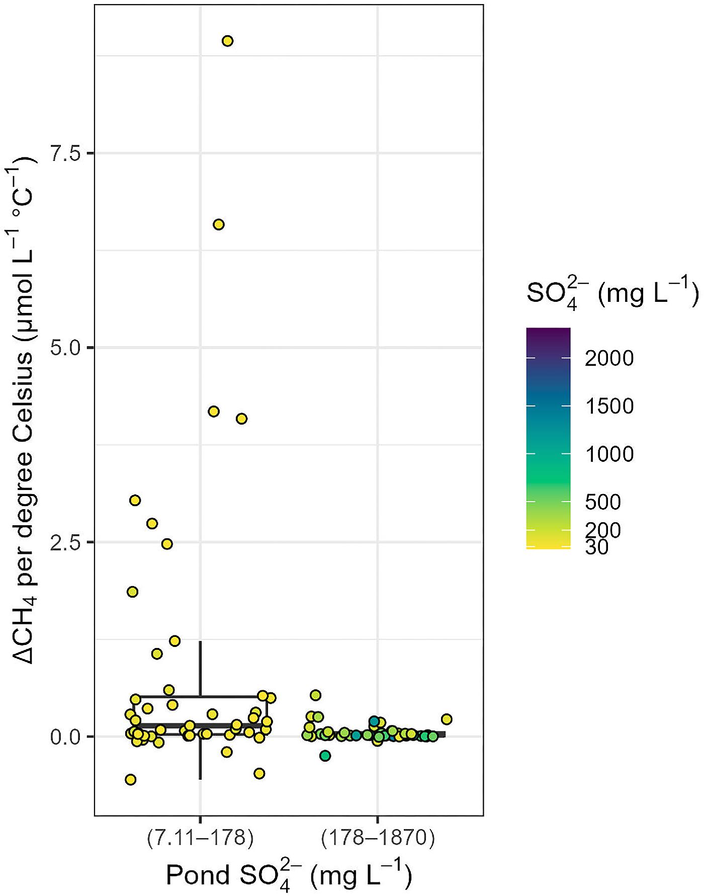
Methane

Methane supersaturation indicates that methanogenesis was occurring in all ponds, and at least 36% of the total variation of ΔCH4 was described by SO42− concentrations. Our results show that at surface water SO42− >178 mg L−1, ΔCH4 concentrations stay close to saturation. Below this threshold, ΔCH4 concentrations are highly variable and difficult to predict based on SO42− alone (Fig. 3a). The CH4–SO42− relationship is discussed in detail below. In addition to SO42− and season, GLS analysis suggests pond pH is also a predictor for ΔCH4. Delta CH4 decreases with increasing pH, which may reflect pond permanence class (as permanent ponds typically have higher pH, conductivity, and SO42−). Wang et al. (1996) summarize various studies that show methane-producing bacteria can have different pH preferences, but there has been no investigation of methanogens and pH in the PPR.
Prairie potholes often have high SO42− concentrations because of the region’s geological parent material (Van Stempvoort et al. 1994) and the closed-basin nature of potholes (Nachshon et al. 2013). In previous prairie pothole research, SO42− has been attributed as an inhibitor of CH4 production, but without determining a specific SO42− concentration at which this effect is important (e.g., Pennock et al. 2010; Bansal et al. 2016; Bortolotti et al. 2016a). While Dalcin Martins et al. (2017) reported the potential for CH4 production via conversion of labile C pools in zones of active SO42− reduction, our field data provide limited evidence that this is occurring at our study sites, as ΔCH4 was consistently low where surface water concentrations indicate a large supply of SO42−. Low ΔCH4 at high SO42− concentrations can be attributed to the more favourable energy yield from SO42− reduction. Inhibition of methanogenesis by SO42− reduction in incubation experiments for ecosystems quite different to PPR ponds suggested substantial methanogenesis limitation at SO42− concentrations >168 mg L−1 (bacteria cultures; Khan and Trottier 1978) and > 240 mg L−1 (lake sediments; Winfrey and Zeikus 1977). These results agree well with the SO42− threshold for methanogenesis identified for ponds in this study, supporting the assumption that this threshold can be applied across the PPR to predict CH4 concentration in ponds and their role in CH4 release to the atmosphere.
Though higher SO42− concentrations appear to inhibit CH4, one pond showed elevated ΔCH4 (8.4 µmol L−1) at relatively high SO42− concentration (2606 mg L−1) in summer (Fig. 3a). This pond had high ΔCH4 in the spring (CH4 concentration was higher than > 75% of all the ponds sampled in spring), and the pond had the largest (evaporation driven) increase of SO42− from spring to summer, with spring concentration of only 235 mg L−1. Of the other ponds with >1000 mg L−1 increase in SO42− concentrations between seasons, some ponds also exhibited CH4 increases of a similar magnitude (∼400%), but they had much lower spring ΔCH4. We hypothesize that methanogenesis occurred primarily before the dramatic increase in SO42− concentrations, and slow or delayed release of this CH4 from sediments to the water column coupled with strong water table drawdown and evaporative concentration yielded uniquely high CH4 for this level of SO42−. Further, SO42− impairment of CH4 production appears to vary widely. In the sewage sludge incubations, CH4 production decreased by no more than 50% at 1150 mg L−1 SO42− (Khan and Trottier 1978), while in freshwater sediment incubations, CH4 production decreased by ∼95% at 960 mg L−1 SO42− (Winfrey and Zeikus 1977), suggesting that some CH4 production is possible across the wide range of SO42− concentrations observed in pothole ponds in this and other studies.
While temperature increases rates of methanogenesis (Wang et al. 1996) and broadly CH4 emissions (e.g., Bansal et al. 2016), temperature explained a very limited amount of variability in ΔCH4 when examined across all sites (Table 4). The effect of temperature on CH4 efflux may be most apparent at sites with consistently high rates of CH4 production, but this effect is not clear for sites where CH4 efflux is lower and variable between years (Baron et al. 2022). In ponds we sampled, temperature likely plays a role in the significant seasonal increase of CH4, as higher CH4 was observed for the same level of SO42− in summer (Fig. 3b) and season was significant in the GLS model, but lower gas solubility at elevated temperature could also be contributing.

Carbon dioxide

The well-known relationship between %CO2 and pH accounted for 50%–80% of %CO2 variation in this study. This relationship is largely driven by the chemical link between CO2 and pH where the dominant forms of dissolved inorganic carbon (DIC) in water, one of which is CO2, depend on H+ activity. Above a pH of 9, dissolved CO2 exists only in small quantities while DIC is dominated by bicarbonate (HCO3) and carbonate (CO32−) (Wetzel 2001). As such, every pond with pH > 9 was undersaturated in CO2, except for one marginally supersaturated site. When pH was less than 9, the link between pH and CO2 does not explain all of the variation seen in levels of CO2 supersaturation. Other studies of inland waters show similar thresholds at pH 9 (Duarte et al. 2008) or somewhat lower (Finlay et al. 2009), with minor variation potentially due to site-specific conditions such as salinity or ecosystem productivity. Biological CO2–pH links (the balance of autotrophy and heterotrophy in the pond) add complexity to determining the mechanism behind the relationship observed here. Notably, we observed higher %CO2 in summer in many ponds despite their higher overall pH. Parameters such as temperature and chl a, which might be expected to exhibit correlation with %CO2, did not.
Other factors that affect the relationship between CO2 saturation and pH include pond alkalinity, pond connection to groundwater (which can be a source of alkalinity), and duration of ice cover. Alkalinity can add dissolved CO2 from calcium carbonate (Wetzel 2001); however, there was no correlation between alkalinity and %CO2 and so does not appear to be important here. Alkalinity and pH were significantly positively correlated (rho = 0.29, p < 0.01, Supplementary Table S4), so buffering capacity may indirectly help to explain %CO2 in PPR ponds. Other variables correlated to %CO2 and investigated for model fit, SO42− and urea, did not show any convincing relationships with the CO2 concentrations in this study (SO42− was more strongly correlated with pH than with ΔCO2). Though seasonal differences for CO2 saturation and fluxes were only weakly significant, there was an almost even split between ponds in which ΔCO2 increased from spring to summer and ponds in which ΔCO2 decreased (Supplementary Fig. S2a). These different behaviours could be linked to pH dynamics over multiple open-water seasons. For example, duration of ice cover on prairie lakes was a key driver for long-term changes in pH because ice cover duration impacted spring pH (Finlay et al. 2015). This multi-year effect could also apply to prairie ponds that retain water or ice over winter. Interestingly, those ponds where ΔCO2 decreased from spring to summer showed an overall increase in pH, while for those where ΔCO2 increased, pH was relatively unchanged from spring to summer (Supplementary Fig. S2b). While pH is clearly important for estimating CO2 saturation in prairie potholes, and our work highlights diverging patterns of pothole behaviour from spring to summer, there remains room for further investigations to provide additional clarity, and detailed temporal investigations at individual ponds may better illustrate site-specific and dynamic processes that our regional analysis does not provide an opportunity to explore.

Nitrous oxide

Nitrous oxide saturation was relatively low, with approximately 60% or more of ponds undersaturated in N2O in both spring and summer, as compared to 45% or less for CO2 and 0% for CH4, and no single physicochemical variable strongly predicted ΔN2O. Spearman rank correlation coefficients indicate significant correlations between ΔN2O and pH and SO42− (Table 3), but we found no suitable linear regression or GLS model for these variables and their relationship with N2O (Table 4). We found no relationship between %N2O and NOx or TAN and it is unclear whether N2O was generated via nitrification, denitrification, or both. Denitrification is often assumed to be the main producer of N2O in aquatic environments, but evidence for this in our results was limited. Because NO3 is required for denitrification, we expected NOx to be a potential predictor of N2O. Research shows that denitrification rates increase with increasing pH (Müller et al. 1980), but the production of N2O by denitrification may be limited by pH >8 (Van Cleemput et al. 1975), representing a large number of our sites, or be specific to the denitrifying bacteria present. In one study, peak production of N2O occurred at pH 7 and 8 for two different species (Burth and Ottow 1983). In our results, %N2O was weakly related to water column pH (rho = 0.28, p <0.01; Table 3) and the highest N2O values occurred where water column pH was below 8.5, but N2O and sediment pH were not related, nor were water column pH and sediment pH (data not shown).
Low ΔN2O and inconclusive relationships between ΔN2O and physicochemical variables could point to dominance of dissimilatory nitrate reduction to ammonia (DNRA) over denitrification for transforming NO3 in potholes. DNRA is favoured by alkaline conditions and SO42−-rich conditions (acting as additional electron acceptors), while denitrification is favoured by pH of 6–8 and is inhibited by high sulfide. DNRA occurs much more rapidly in prairie potholes than denitrification (Hergott 2022), and preference for this N transformation pathway could contribute to the undersaturation of N2O observed for the majority of sites and the absence of a relationship between NO3 and ΔN2O. Additionally, since all ponds had less than 1 mg L−1 NO3 (and lower TAN and urea concentrations), available NO3 may be quickly taken up and incorporated as organic N rather than used in denitrification, as pelagic N uptake rates have been shown to be very high for ponds in the region (Hergott 2022). Having very few ponds with elevated ΔN2O or large N2O efflux (i.e., data were highly positively skewed) presented a challenge in our analysis.

GHG fluxes and the radiative balance

Multiple studies in the PPR have investigated fluxes of GHG in potholes, but only some consider the open water areas in detail, and these are often limited to small numbers of sites or a select GHG. Studies that focus on open water in prairie potholes show that diffusive CH4 and CO2 effluxes in the open-water season are typical (Badiou et al. 2011; Bortolotti et al. 2016a). Meanwhile, N2O undersaturation (or negative flux) is common, but pothole ponds have small N2O effluxes on average (Tangen and Bansal 2022). Small agricultural reservoirs in the region exhibited very similar diffuse GHG flux behaviour (Webb et al. 2019a, 2019b).
Mean diffusive GHG fluxes for ponds in this study are comparable to the few available studies of ponded zone GHG fluxes for pothole ponds (Table 7). Our results show somewhat higher average N2O release to the atmosphere, but lower CH4 and CO2 release rates. Our mean GHG fluxes were usually lower than GHG fluxes from studies that included pothole pond basins (Table 7), though there are important methodological differences that are discussed below. Pond-diffusive GHG fluxes in this study aligned well with mean fluxes from agricultural reservoirs and global estimates of CO2 and CH4 fluxes from ponds or small lakes (Table 7).
Table 7.
Table 7. Mean diffusive GHG fluxes estimated in this study compared to other studies in the Prairie Pothole Region (PPR) in Canada (CA) and the United States (US).
      Mean diffuse fluxes  
Flux sourceLocationSampling year (s)Sites (n)Surface areac (m2)Study typeN2O (µmol m−2 d−1)CO2 (mmol m−2 d−1)CH4 (mmol m−2 d−1)Flux methodStudy
Pothole pondAlberta, Saskatchewan, Manitoba, CAApril/May, June/July 201915728–1900survey1.9522.8Headspace equilibrium, k from wind modelThis study
Pothole pondSaskatchewan, CAMay–September, 201332670–8750intensiveNA834.9Headspace equilibriumBortolotti et al. (2016a)
Pothole pondNorth Dakota, USMay–October, 20152 intensiveNA607.0Static chamberDalcin Martins et al. (2017)
Pothole pondMontana, N. Dakota, S. Dakota, Minnesota, Iowa, USApril–September 2003–2016177 (ranging from 12 to 119 each year)40 000–190 000 (incl. upland)intensive1.0NANAStatic chamberTangen and Bansal (2022)
Pothole basinaAlberta, Saskatchewan, Manitoba, CAApril–October, 2004–200562NAsurvey + intensive9.9NA1.5Static chamberBadiou et al. (2011)
Pothole basinbNorth Dakota, Minnesota, Iowa, USApril–September, 2005–2008119 (with 41 sites for 2007–08)2100–18800intensive14NA69Static chamberTangen et al. (2015)
Small agricultural reservoirSaskatchewan, CAJuly–August, 2017101158–13900survey1.5447.1Headspace equilibrium, measured kWebb et al. (2019a, 2019b)
Global pond/lake estimatePondsVarious studies50<1000reviewNA352.3Headspace equilibrium, k from lake-sizeHolgerson and Raymond (2016)
Global pond/lake estimatePondsVarious studies221000–10000reviewNA210.65Headspace equilibrium, k from lake-size Holgerson and Raymond (2016)

Note: We include one global estimate of CO2 and CH4 fluxes for additional context. Differences between GHG flux estimates can be caused by different methods and study designs.

a
Pothole basin = riparian zone, wet edge, and centre of the basin. Fluxes are aggregate of these three landscape elements (Badiou et al. 2011).
b
Pothole basin = five positions from slope inflection (upland–wetland boundary) to the basin centre (see Fig. 2, Finocchiaro et al. 2014). Fluxes are an area-weighted average.
c
Note that studies have each reported surface area in slightly different ways; this column is included for rough comparison.
Differences between our results and other studies reported here can arise due to differences in where, how, and when we sampled ponds. We sampled a large number of sites, during only two measurement periods and for a single year during a dry climate phase in the region when many ponds dried out in early or mid summer. Because we investigated only ponded areas, we would expect smaller year-to-year differences than investigations of wetland basins as a whole for which extent of inundated areas and moisture conditions can affect fluxes (Tangen and Bansal 2022). Interannual differences at the whole pond basin level can be large (Badiou et al. 2011); thus, differences between studies could reasonably be due to interannual variability in biogeochemical or hydrologic conditions. Additionally, our approach to quantifying GHG fluxes (wind-based model) provides an estimate of fluxes, and these estimates can be affected by wind conditions at the time of sampling and by the model used to approximate gas transfer velocity (Supplementary Fig. S1). On the other hand, chamber measurements used in many other studies are also subject to some limitations (e.g., Lorke et al. 2015), so methodologies can contribute to differences in estimates between studies.Bortolotti et al. (2016a) and Dalcin Martins et al. (2017) focused on a few ponds (n = 3 and n = 2, respectively) with more temporal measurements, including sampling later into the warmer part of the open water season, which could be another reason why they reported higher mean CH4 and CO2 flux rates for their sites. Tangen et al. (2015) also reported higher mean GHG fluxes, but these fluxes combine measurements from open water and the surrounding vegetation and dry land (weighted by area), making it difficult to compare to our results. Dry areas likely have a large impact on GHG fluxes from potholes; efflux of CH4 and N2O (Gleason et al. 2009; Tangen and Bansal 2022) and CO2 (DelVecchia et al. 2019) from drying sediments was greater than from open water for restored pothole ponds and alpine wetlands, respectively.
Median CO2-eq fluxes in this study suggest that many ponds could be sources in the global GHG budget (Table 6). Methane was an important contributor to CO2-eq fluxes for these ponds, making up 46% and 71% of CO2-eq on average for 100 and 20-yr GWP periods, respectively. Methane emissions from small ponds are recognised as globally significant, whether they are grouped with wetland CH4 emissions (Wang et al. 1996; Canadell et al. 2021) or lakes and reservoirs with surface area ranging from 0.01 to 10 000 km2 (DelSontro et al. 2018). Our results suggest that CH4 can play an important role for pothole pond diffusive contributions to radiative balance in the region. It is notable that CH4 held such importance without including what is expected to be the dominant CH4 emission pathway (ebullition), for which flux to the atmosphere can be much higher (Baron et al. 2022). However, diffusive GHG efflux was also relatively low for many ponds, evidenced by how mean GHG fluxes compared to other studies (Table 7). Uptake of CO2 by emergent plants is expected to offset some or all of CO2 efflux but we did not quantify this, and coverage of emergent vegetation was highly variable in the ponds we sampled.
Considering that CH4 efflux was a major contributor to CO2-eq flux and significantly increased from spring to summer in this study, warming regional temperatures increase the potential for CH4 efflux from potholes during ponded conditions. In future climate scenarios, CH4 efflux from prairie potholes (from ponded or other wetland areas) is expected to increase (Bansal et al. 2023), though there are likely differences between ponds. For example, CH4 efflux from permanent ponds was less sensitive to changes in temperature or water depth than temporary ponds (Bansal et al. 2016). Here we show that ΔCH4 response to temperature increase is approximately an order of magnitude higher when SO42− concentrations are below the 178 mg L−1 threshold we identified as important to CH4 saturation levels (Fig. 4). In this study, 52% of ponds had a mean SO42− concentration below 178 mg L−1 and 48% had higher mean SO42−. Note that our sampling was biased against including large ponds (typically more saline) because sites were selected from bird habitat surveys. Since SO42− concentration typically is higher in permanent or semi-permanent ponds than in seasonal or temporary ponds, our findings support that pond response to temperature increase will not be uniform.
Fig. 4.
Fig. 4. Change in ΔCH4 (µmol L−1) per degree of temperature change (°C) for ponds with mean SO42− concentrations that are low (7.11–178 mg L−1) or high (178–1870 mg L−1). The median change in dissolved CH4 for ponds with low SO42− was 0.14 µmol L−1 °C−1, while the median change for ponds with high SO42− was 0.019 µmol L−1 °C−1.
Despite their importance as sites of C storage, the role of pothole ponds in the global radiative balance is complex. Open-water areas of seasonal to permament pothole ponds have the potential to be positive feedbacks on climate through diffusive exchange with the atmosphere. Methane emissions are important in this regard, but with the potential for CO2 and N2O uptake to partly negate this for some ponds. Moreover, ponds with high SO42− concentration have lower levels of CH4 supersaturation (Fig. 3), and can be expected to have more muted response to increases in temperature (Fig. 4).

Conclusions

We quantified ΔGHG concentrations and diffusive GHG fluxes for a large number of ponds capturing much of the naturally occurring variability across the Canadian PPR, and show that diffusive GHG fluxes are necessary to consider when estimating long-term C storage potential of potholes in the context of changing climate. Ponds were always supersaturated with CH4, close to split between undersaturated and supersaturated with CO2, and usually undersaturated with N2O. Overall, the physicochemical parameters SO42− and pH were good individual predictors of CH4 and CO2, respectively, but we found no clear predictor of N2O. The relationships between GHGs and physicochemical parameters identified here are expected to hold across similar systems of the PPR. Seasonal change was very important for pond physicochemical conditions and is linked to pond hydrological function and processes. Delta CH4 increased strongly from spring to summer sampling periods and, as the dominant contributor to GWP from diffusive emissions in these systems, was a major reason for the 5-fold increase in diffusive emissions as CO2-eq from spring to summer.
Future work should aim to capture more ponds with supersaturated N2O conditions, investigate finer temporal dynamics and additional physicochemical parameters like DO, and have longer sampling periods. Since pond hydrologic conditions change from year to year and biogeochemical behaviour can be altered by agricultural practices, multi-year studies of GHG dynamics are key. There remain important unknowns about the transient nature of these systems when inundated areas no longer hold water during prolonged dry phases of regional climate. Multi-year studies also would be relevant for understanding the impacts to pond ecosystem services from climate change and the consequences of those impacts for society.

Acknowledgements

This work would not have been possible without the invaluable support of K. Nugent, C. Hoggarth, and the Prairie Water team who supported the survey, including C. Morrissey and members of her lab. This work was funded in part by an NSERC Discovery Grant and CFREF (Global Water Futures) sub-grant (Prairie Water) held by CJW. LTM was supported in part by an NSERC CGS. We appreciate comments from L. Bortolotti, J. Venkiteswaran, and K. Finlay on earlier drafts of this work that helped us to improve the work.

References

Arts M.T., Robarts R.D., Kasai F., Waiser M.J., Tumber V.P., Plante A.J., et al. 2000. The attenuation of ultraviolet radiation in high dissolved organic carbon waters of wetlands and lakes on the northern Great Plains. Limnology and Oceanography, 45: 292–299.
Arya S.P. 2001. Introduction to micrometeorology. 2nd ed. Edited by J.R Holton. Academic Press, New York. 446p.
Badiou P., McDougal R., Pennock D., Clark B. 2011. Greenhouse gas emissions and carbon sequestration potential in restored wetlands of the Canadian prairie pothole region. Wetlands Ecology and Management, 19(2): 237–256.
Bansal S., Post van der Burg M., Fern R.R., Jones J.W., Lo R., McKenna O.P., et al. 2023. Large increases in methane emissions expected from North America's largest wetland complex. Science Advances. 9: eade1112.
Bansal S., Tangen B., Finocchiaro R., 2016. Temperature and hydrology affect methane emissions from Prairie pothole wetlands. Wetlands, 36(Suppl 2): 371.
Baron A.A.P., Dyck L.T., Amjad H., Bragg J., Kroft E., Newson J., Oleson K., et al. 2022. Differences in ebullitive methane release from small, shallow ponds present challenges for scaling. Science of the Total Environment, 802: 149685.
Bortolotti L.E., St. Louis V.L., Vinebrooke R.D. 2019. Drivers of ecosystem metabolism in restored and natural prairie wetlands. Canadian Journal of Fisheries and Aquatic Sciences, 76: 2396–2407.
Bortolotti L.E., St. Louis V.L., Vinebrooke R.D., Wolfe A.P. 2016a. Net ecosystem production and carbon greenhouse gas fluxes in three Prairie wetlands. Ecosystems 19: 411–425.
Bortolotti L.E., Vinebrooke R.D., St. Louis V.L. 2016b. Prairie wetland communities recover at different rates following hydrological restoration. Freshwater Biology, 61: 1874–1890.
Burth I., Ottow J.C.G. 1983. Influence of pH on the production of N₂O and N₂ by different denitrifying bacteria and fusarium solani. Ecological Bulletins, 35: 207–215. Available from http://www.jstor.org/stable/20112855.
Canadell J.G., Monteiro P.M.S., Costa M.H., Cotrim da Cunha L., Cox P.M., Eliseev A.V, et al. 2021. Global carbon and other biogeochemical cycles and feedbacks. In Change 2021: The Physical Science Basis. Contribution of Working Group I to the Sixth Assessment Report of the Intergovernmental Panel on Climate Change. Edited by V. Masson-Delmotte, P. Zhai, A. Pirani, S.L. Connors, C. Péan, S. Berger, et al. Cambridge University Press, Cambridge, United Kingdom and New York, NY. pp. 673–816.
Cole J.J., Caraco N.F. 1998. Atmospheric exchange of carbon dioxide in a low-wind oligotrophic lake measured by the addition of SF6. Limnology & Oceanography. 43(4): 647–656.
Coplen T.B. 1996. New guidelines for reporting stable hydrogen, carbon, and oxygen isotope-ratio data. Geochimica et Cosmochimica Acta. 60(17): 3359–3360.
Dalcin Martins P.D., Hoyt D.W., Bansal S., Mills C.T., Tfaily M., Tangen B.A., et al. 2017. Abundant carbon substrates drive extremely high sulphate reduction rates and methane fluxes in prairie pothole wetlands. Global Change Biology, 23: 3107–3120.
Dansgaard W. 1964. Stable isotopes in precipitation. Tellus, 16(4): 436–468.
DelSontro T., Beaulieu J.J., Downing J.A. 2018. Greenhouse gas emissions from lakes and impoundments: upscaling in the face of global change. Limnology & Oceanography Letters, 3: 64–75.
DelVecchia A.G., Balik J.A., Campbell S.K., Taylor B.W., West D.C., Wissinger S.A. 2019. Carbon dioxide concentrations and efflux from permanent, semi-permanent, and temporary subalpine ponds. Wetlands, 39: 955–969.
Downing J.A. 2010. Emerging global role of small lakes and ponds: little things mean a lot. Limnetica, 29(1): 9–24.
Downing J.A., Prairie Y.T., Cole J.J., Duarte C.M., Tranvik L.J., Striegl R.G., et al. 2006. The global abundance and size distribution of lakes, ponds and impoundments. Limnology and Oceanography. 51(5): 2388–2397.
Duarte C.M., Prairie Y.T., Montes C., Cole J.J., Striegl R., Melack J., et al. 2008. CO2 emissions from saline lakes: a global estimate of a surprisingly large flux. Journal of Geophysical Research, 113: 1–7.
Euliss N.H., Gleason R.A., Olness A., McDougal R.L., Murkin H.R., Robarts R.D., et al. 2006. North American prairie wetlands are important nonforested land-based carbon storage sites. Science of the Total Environment, 361: 179–188.
Finlay K., Leavitt P.R., Wissel B., Prairie Y.T. 2009. Regulation of spatial and temporal variability of carbon flux in six hard-water lakes of the Northern Great Plains. Limnology & Oceanography. 54(6, part 2): 2553–2564.
Finlay K., Vogt R.J., Bogard M.J., Wissel B., Tutolo B.M., Simpson G.L., et al. 2015. Decrease in CO2 efflux from northern hardwater lakes with increasing atmospheric warming. Nature, 519: 215–218.
Finocchiaro R., Tangen B., Gleason R. 2014. Greenhouse gas fluxes of grazed and hayed wetland catchments in the U.S. Prairie Pothole Ecoregion. Wetlands Ecology and Management, 22: 305–324.
Forster P., Storelvmo T., Armour K., Collins W., Dufresne J.-L., Frame D., et al. 2021. The Earth's energy budget, climate feedbacks, and climate sensitivity. In Climate Change 2021: The Physical Science Basis. Contribution of Working Group I to the Sixth Assessment Report of the Intergovernmental Panel on Climate Change. Edited by V. Masson-Delmotte, P. Zhai, A. Pirani, S.L. Connors, C. Péan, S. Berger, et al. Cambridge University Press, Cambridge, United Kingdom and New York, NY. pp. 923–1054.
Fox J., Weisberg S. 2019. An R companion to applied regression. 3rd ed. Sage, Thousand Oaks, CA.
Gibson J.J., Edwards T.W.D., Birks S.J., St Amour N.A., Buha W.M., McEachern P., et al. 2005. Progress in isotope tracer hydrology in Canada. Hydrological Processes, 19: 303–327.
Gleason R.A., Tangen B.A., Browne B.A., Euliss N.H. 2009. Greenhouse gas flux from cropland and restored wetlands in the Prairie Pothole Region. Soil Biology and Biochemistry. 41: 2501–2507.
Harrell F.Jr. 2023. Hmisc: Harrell Miscellaneous. R package version 5.1-1. Available from https://cran.r-project.org/package=Hmisc.
Hayashi M., van der Kamp G., Rosenberry D.O. 2016. Hydrology of prairie wetlands: understanding the integrated surface-water and groundwater processes. Wetlands, 36(Suppl 2): 237.
Hergott A.E. 2022. Prairie potholes as transformers on the landscape: exploring the rates of planktonic nitrogen uptake, DNRA, and denitrification. M.E.S thesis, University of Saskatchewan, Saskatoon, Saskatchewan. 111 p.
Holgerson M.A., Raymond P.A. 2016. Large contribution to inland water CO2 and CH4 emissions from very small ponds. Nature Geoscience, 9: 222–226.
Jafari M., Ansari-Pour N., 2019. Why, when and how to adjust your p values? Cell Journal, 20(4): 604–607.
Jähne B.J., Münnich K.O.M., Bösinger R., Dutzi A., Huber W., Libner P. 1987. On the parameters influencing air-water gas exchange. Journal of Geophysical Research, 92(C2): 1937–1949.
Jasechko S. 2019. Global isotope hydrogeology―review. Reviews of Geophysics, 57: 835–965.
Khan A.W., Trottier T.M. 1978. Effect of sulfur-containing compounds on anaerobic degradation of cellulose to methane by mixed cultures obtained from sewage sludge. Applied and environmental microbiology, 35(6): 1027–1034.
Kirschke S., Bousquet P., Ciais P., Saunois M., Canadell J.G., Dlugokencky E.J., et al. 2013. Three decades of global methane sources and sinks. Nature Geoscience, 6: 813–823.
LaBaugh J.W. 1989. Chemical characteristics of water in Northern Prairie wetlands. In Northern Prairie Wetlands. Edited by A. van der Valk. Iowa State University Press, Ames, Iowa. pp. 56–90.
LaBaugh J.W., Winter T.C., Rosenberry D.O. 1998. Hydrologic functions of Prairie wetlands. Great Plains Research, 8(1): 17–37.
Lin Pedersen T. 2024. ggforce: Accelerating 'ggplot2'. R package version 0.4.2. Available from https://CRAN.R-project.org/package=ggforce
Lorke A., Bodmer P., Noss C., Alshboul Z., Koschorreck M., Somlai-Haase C., et al. 2015. Technical note: Drifting versus anchored flux chambers for measuring greenhouse gas emissions from running waters. Biogeosciences, 12 (23): 7013–7024.
McDonald J.H. 2014. Handbook of biological statistics. 3rd ed. Sparky House Publishing, Baltimore, MD.
McFarlan L. 2021. Where's the P in prairie potholes? Identifying patterns of phosphorus accumulation in Canadian Prairie wetlands. M.E.S. thesis, University of Saskatchewan, Saskatoon, Saskatchewan. 86p.
Mitsch W.J., Gosselink J.G. 2015. Wetlands. 5th ed. John Wiley & Sons, Inc. Hoboken, NJ. pp. 736.
Müller M.M., Sundman V., Skujinš J. 1980. Denitrification in low pH spodosols and peats determined with the acetylene inhibition method. Applied and environmental microbiology, 40(2): 235–239.
Nachshon U., Ireson A., van der Kamp G., Wheater H. 2013. Sulphate salt dynamics in the glaciated plains of North America. Journal of Hydrology, 499: 188–199.
Neubauer S.C. 2021. Global warming potential is not an ecosystem property. Ecosystems, 24: 2079–2089.
Pennock D., Yates T., Bedard-Haughn A., Phipps K., Farrell R., McDougal R. 2010. Landscape controls on N2O and CH4 emissions from freshwater mineral soil wetlands of the Canadian Prairie Pothole region. Geoderma, 155: 308–319.
Petrescu A.M.R., Lohila A., Tuovinen J.-P., Baldocchi D.D., Desai A.R., Roulet N.T., et al. 2015. The uncertain climate footprint of wetlands under human pressure. Proceedings of the National Academy of Sciences of the United States of America 112(15): 4594–4599.
Pfahl S., Sodemann H. 2014. What controls deuterium excess in global precipitation? Climate of the Past, 10(2): 771–781.
Pinheiro J., Bates D., R Core Team. 2021. nlme: linear and nonlinear mixed effects models R package version 3.1-163. Available from https://cran.r-project.org/web/packages/nlme/index.html
Post van der Burg M., Tangen B.A. 2015. Monitoring and modeling wetland chloride concentrations in relationship to oil and gas development. Journal of Environmental Management, 150: 120–127.
R Core Team. 2023. R: a language and environment for statistical computing. R Foundation for Statistical Computing, Vienna. Available from https://www.R-project.org/
Ruso G.E., Morrissey C.A., Hogan N.S., Sheedy C., Gallant M.J., Jardine T.D. 2019. Detecting amphibians in agricultural landscapes using environmental DNA reveals the importance of wetland condition. Environmental Toxicology and Chemistry, 38(12): 2750–2763.
Schlesinger W.H., Bernhardt E.S. 2020. Biogeochemistry: an analysis of global change, 4th ed. Academic Press, London. 749p.
Sebacher D.I., Harriss R.C., Bartlett K.B. 1983. Methane flux across the air-water interface: air velocity effects. Tellus B: Chemical and Physical Meteorology, 35B: 103–109.
Spence C., Wolfe J.D., Whitfield C.J., Baulch H.M., Basu N.B., Bedard-Haughn A.K., et al. 2019. Prairie water: a global water futures project to enhance the resilience of prairie communities through sustainable water management. Canadian Water Resources Journal / Revue canadienne des ressources hydriques. 44(2): 115–126.
St Amour N.A., Gibson J.J., Edwards T.W.D., Prowse T.D., Pietroniro A. 2005. Isotopic time-series partitioning of streamflow components in wetland-dominated catchments, lower Liard River basin, Northwest Territories, Canada. Hydrological Processes, 19(17): 3357–3381.
Stewart R.E., Kantrud H.A. 1971. Classification of natural ponds and lakes in the glaciated prairie region. Resource Publication 92. Bureau of Sport Fisheries and Wildlife, Washington, D.C. p. 57.
Tangen B.A., Bansal S. 2022. Prairie wetlands as sources or sinks of nitrous oxide: Effects of land use and hydrology. Agricultural and Forest Meteorology, 320: 108968.
Tangen B.A., Finocchiaro R.G., Gleason R.A. 2015. Effects of land use on greenhouse gas fluxes and soil properties of wetland catchments in the Prairie Pothole Region of North America. Science of the Total Environment, 533: 391–409.
Tranvik L.J., Downing J.A., Cotner J.B., Loiselle S.A., Striegl R.G., Ballatore T.J., et al. 2009. Lakes and reservoirs as regulators of carbon cycling and climate. Limnology & Oceanography, 54(6): 2298–2314.
Van Cleemput O., Patrick W.H.J., McIlhenny R.C. 1975. Formation of chemical and biological denitrification products in flooded soil at controlled pH and redox potential. Soil Biology and Biochemistry, 7: 329–332.
Van Stempvoort D.R., Hendry M.J., Shoenau J.J., Krouse H.R. 1994. Sources and dynamics of sulfur in weathered till, Western Glaciated Plains of North America. Chemical Geology, 111: 35–56.
Wang Z., Deng Z., Patrick W.H. Jr. 1996. Methane emissions from natural wetlands. Environmental Monitoring and Assessment, 42: 143–161.
Wanninkhof R. 1992. Relationship between wind speed and gas exchange over the ocean. Journal of Geophysical Research, 97(C5): 7373–7382.
Webb J.R., Hayes N.M., Simpson G.L., Leavitt P.R., Baulch H.M., Finlay K. 2019a. Widespread nitrous oxide undersaturation in farm waterbodies creates an unexpected greenhouse gas sink. Proceedings of the National Academy of Sciences of the United States of America, 116(20): 9814–9819.
Webb J.R., Leavitt P.R., Simpson G.L., Baulch H.M., Haig H.A., Hodder K.R., Finlay K., 2019b. Regulation of carbon dioxide and methane in small agricultural reservoirs: optimizing potential for greenhouse gas uptake. Biogeosciences, 16, 4211–4227.
Weiss R.F., Price B.A. 1980. Nitrous oxide solubility in water and seawater. Marine Chemistry, 8: 347–359.
Wetzel R.G. 2001. Limnology: lake and river ecosystems. 3rd ed. Academic Press, San Diego, CA. p. 1006.
Whitfield C.J., Aherne J., Baulch H.M. 2011. Controls on greenhouse gas concentrations in polymictic headwater lakes in Ireland. Science of the Total Environment, 410-411: 217–225.
Wickham H. 2016. ggplot2: Elegant graphics for data analysis. Springer-Verlag, New York.
Wilke C.O. 2020. cowplot: Streamlined plot theme and plot annotations for 'ggplot2'. R package version 1.1.3. Available from https://cran.r-project.org/web/packages/cowplot/index.html
Wilke C.R., Chang P. 1955. Correlation of diffusion coefficients in dilute solutions. AIChE Journal, 1(2): 264–270.
Winfrey M.R., Zeikus J.G. 1977. Effect of sulphate on carbon and electron flow during microbial methanogenesis in freshwater sediments. Applied and environmental microbiology, 33(2): 275–281.
Winter T., 1989. Hydrologic studies of wetlands in the northern prairies. In Northern Prairie Wetlands. Edited by A. van der Valk. Iowa State University Press, Ames, IA. pp. 16–54.
Yamamoto S., Alcauskas J.B., Crozier T.E. 1976. Solubility of methane in distilled water and seawater. Journal of Chemical and Engineering Data, 21(1): 78–80.

Supplementary material

Supplementary Material 1 (DOCX / 265 KB).

Information & Authors

Information

Published In

cover image FACETS
FACETS
Volume 9January 2024
Pages: 1 - 18
Editor: Nora Jessie Casson

History

Received: 31 July 2023
Accepted: 15 January 2024
Version of record online: 25 June 2024

Notes

This paper is one of a collection entitled Canadian biogeoscience research in the food-water-energy nexus: advances from processes to modelling.

Data Availability Statement

Data generated and analyzed during this study are available from the corresponding author upon request.

Key Words

  1. Prairie Pothole Region
  2. methane
  3. carbon dioxide
  4. nitrous oxide
  5. sulfate
  6. pH

Sections

Subjects

Plain Language Summary

Investigating greenhouse gases in small prairie ponds: do season and water chemistry matter?

Authors

Affiliations

Global Institute for Water Security, University of Saskatchewan, SK, Canada
School of Environment and Sustainability, University of Saskatchewan, SK, Canada
Author Contributions: Conceptualization, Data curation, Formal analysis, Methodology, Writing – original draft, and Writing – review & editing.
Global Institute for Water Security, University of Saskatchewan, SK, Canada
School of Environment and Sustainability, University of Saskatchewan, SK, Canada
Author Contributions: Conceptualization, Methodology, and Writing – review & editing.
Colin J. Whitfield served as Guest Editor at the time of manuscript review and acceptance and did not handle peer review and editorial decisions regarding this manuscript.

Author Contributions

Conceptualization: LTM, CJW
Data curation: LTM
Formal analysis: LTM
Methodology: LTM, CJW
Writing – original draft: LTM
Writing – review & editing: LTM, CJW

Competing Interests

The authors declare there are no competing interests.

Metrics & Citations

Metrics

Other Metrics

Citations

Cite As

Export Citations

If you have the appropriate software installed, you can download article citation data to the citation manager of your choice. Simply select your manager software from the list below and click Download.

There are no citations for this item

View Options

View options

PDF

View PDF

Get Access

Media

Media

Other

Tables

Share Options

Share

Share the article link

Share on social media