Bull kelp (Nereocystis luetkeana) growth rates as climate stress indicators for Canada’s Pacific coast
Abstract
Primary producers’ growth rates are ideal bioindicators of changing climate due to their sensitivity to environmental conditions. On the Central Coast of British Columbia, we assessed growth rates of Nereocystis luetkeana, a canopy-forming annual kelp, by assessing baseline variability in growth rates and their response to environmental conditions of over 600 individuals and across three sites (2016–2019). Optimal growth rates for blades and stipes (∼13–14 cm/day) occurred within a narrow range of local environmental conditions. Growth decreased at temperatures > 10 °C, below 1 µm/L nitrate concentration, and surface light availability reduced blade growth at low and high levels (daily light integral or DLI <20 and >40 mol/m2/day). Spatiotemporal variability in these environmental drivers co-occurred with differences in growth rates, suggesting that local conditions strongly influenced growth. In particular, temperature and nutrients were un-coupled seasonally in this region, with more variable responses in growth over the primary growing season (May to September). Overall, the sensitivity of the growth rates of this annual kelp to changing climatic conditions suggests that it is a useful bioindicator for management and marine planning efforts (e.g., restoration and aquaculture) across its species range and provides a feasible metric for monitoring.
Introduction
Biological indicators (“bioindicators”) include species, communities and/or organismal processes used by monitoring and management programs to detect change in population and ecosystem attributes, including ecological functions. These may range across different scales, from habitat forming species to entire ecosystems (Carignan and Villard 2002). Effective bioindicators are generally (1) sensitive to changes in the environment, while remaining stable in response to natural spatial and temporal variability; (2) occupy a temporal and spatial distribution for widespread implementation and comparison; and (3) are feasible and cost-effective to consistently measure (Carignan and Villard 2002; Manickavasagam et al. 2019). Identifying and quantifying the magnitude of directional change and variability in biological indicators in response to anthropogenic stressors or management actions requires assessing the relationships between bioindicators and environmental conditions. Given interannual variability in environmental conditions, multiple years of concurrent environmental data and bioindicator monitoring are often needed to establish these relationships in situ (Morris et al. 2008). Furthermore, understanding the effects of environmental conditions on bioindicators may require advanced statistical modeling of the relationships (Compagnoni et al. 2021). This necessary step is difficult to establish in challenging coastal and marine ecosystems, where in-situ data are logistically challenging to collect.
Given the ecological importance and recent local declines in kelp forests around the globe, there is growing interest in using kelp, and metrics of kelp, as bioindicators of environmental change in marine ecosystems (e.g., Marine Planning Partnership Initiative 2015—Central Coast Marine Plan). Kelp habitats have been shown to be increasingly sensitive to climatic conditions such as temperature, including temperature anomalies and marine heatwaves, long-duration climate-driven fluctuations (e.g., ENSO), and gradual climate warming (Reed et al. 2016; Cavanaugh et al. 2019; Wernberg et al. 2019; Starko et al. 2022). These documented changes in response to climate also impact the ecological functions of kelp forests, including their global role in primary productivity (Mann 1973). Kelp biomass and productivity support diverse assemblages of invertebrates, fishes, mammals, and birds, including many important fisheries and at-risk species (e.g., Mann 1973; Steneck et al. 2002) and serve an important role in nutrient cycling, including nitrogen and carbon uptake via photosynthesis (Teagle et al. 2017; Eger et al. 2023). In Canada, for example, bioindicators are being assessed for monitoring and management of marine ecosystems, led by kelp forest programs among Indigenous stewardship, First Nations and the Province of B.C. (Marine Plan Partnership or MaPP for the North Pacific Coast—Central Coast Annual Report 2020), as well as ecologically significant species (ESS) within ecologically and biologically significant areas (EBSAs) for Fisheries and Oceans (Rubidge et al. 2020).
The use of kelps as bioindicators has led to additional questions about which demographic or functional properties (e.g., kelp growth, biomass, productivity) are most sensitive to environmental change, and therefore serve as the “best” bioindicator. Kelps exhibit rapid rates of growth and recruitment, which are sensitive to seasonal and interannual changes in climate, and result in high biomass turnover and rapid shifts in productivity (e.g., Krumhansl et al. 2016; Wernberg et al. 2019). Consequently, changes in these rates can be used as indicators of interannual and seasonal changes in kelp productivity and health in response to climate-influenced abiotic conditions (Compagnoni et al. 2021). Kelp population-level change in response to the marine environment usually uses information on extent (often for canopy-forming species) and abundance (e.g., densities or % cover). However, demographic parameters or vital rates (e.g., recruitment, mortality and survival) may provide ideal indicators of overall population success. Kelp growth, which is particularly efficient and cost-effective to measure and monitor in situ over time, may therefore serve as an important bioindicator to assess population-level shifts in response to changes in environmental conditions.
Nereocystis luetkeana, bull kelp is an abundant annual canopy-forming laminarian in the northeast Pacific that exhibits dramatic seasonal variability in growth and survival (Foreman 1984; Dobkowski et al. 2019). This life history strategy likely predisposes this species to exhibit different responses to climate change-driven shifts in environmental factors (e.g., light, nutrients, wave action) relative to those of co-occurring perennial kelps such as Macrocystis pyrifera and Pterygophora californica (Dayton et al. 1984; Hamilton et al. 2020; Compagnoni et al. 2021). While some perennial species may be able to persist in the face of episodic extreme events (e.g., Macrocystis pyrifera; (Reed et al. 2016; Cavanaugh et al. 2019) the dynamics of annual species often react more directly to climate volatility as observed in many autotrophs including species of terrestrial grasses, aquatic angiosperms, and macroalgae (e.g., Duarte 1989; Lee et al. 2007; Morris et al. 2008; Straub et al. 2019; Reich et al. 2020; Compagnoni et al. 2021).
In the northeast Pacific, recent collapses in annual populations of N. luetkeana as well as other species of kelps are attributed not only to shifts in herbivory but also to rapid changes in the abiotic conditions that support them, partly as a result of declines in growth (e.g., Berry et al. 2021; McPherson et al. 2021; García-Reyes et al. 2022; Starko et al. 2022). The combined impacts of multiple stressors on kelp, however, can be context specific to kelp life history strategies and the local coastal environment. Kelp declines have been attributed to changes in both abiotic and biotic conditions, including rising sea surface temperatures and anomalies (Wernberg et al. 2013), changes in nutrients and light regime associated with turbidity (Coleman et al. 2008), increasing wave action and storms (Smale and Vance 2016), and loss of predators and overgrazing by herbivores (e.g., Burt et al. 2018). In many, if not most coastal settings, multiple stressors co-occur and influence kelp populations (e.g., Burt et al. 2018; Rogers-Bennett and Catton 2019).
N. luetkeana experiences a wide range of environmental conditions across its broad geographic distribution from central California to subarctic waters of southeast Alaska, which spans a latitudinal temperature gradient of 4 °C to 15 °C (Lüning and Freshwater 1988). Driven by weather patterns, currents and local geography, microclimates also result in substantial variability in temperature, nutrients, and light of N. luetkeana (Foreman 1984). Field observation has documented declines in abundance (Berry et al. 2021) and in photosynthetic performance (Wheeler et al. 1984) in association with changes in abiotic factors such as temperature and dissolved inorganic nitrogen (nitrate). Laboratory studies also suggest that N. luetkeana growth is sensitive to small changes in temperature (Supratya et al. 2020; Fales et al. 2023), nutrients (Ahn et al. 1998), and light (Wheeler et al. 1984). These variable local conditions likely influence N. luetkeana growth dynamics across seasons and years (Brown et al. 1997), as well as the sensitivity of its growth metrics to changing conditions (Foreman 1984), and its ability to adapt to future changes associated with climate stress. Despite the importance of N. luetkeana as a dominant canopy-forming kelp, the effects of specific abiotic conditions on its growth and productivity have not been widely characterized, except for the few focal studies above.
Patterns of persistence in N. luetkeana and other kelps in BC may also differ from those of other regions due to differences in climatic conditions during their primary growing season. Temperature and nutrients in California are correlated through the primary growing season of the dominant canopy-forming perennial kelp, Macrocystis pyrifera (e.g., Zimmerman and Kremer 1984), and both sea surface temperature and nutrient availability are related to the annual recovery of this kelp species in the early spring, with weaker negative relationships spanning the full year (Cavanaugh et al. 2011). As observed through a 25 year times series in California, interannual relationships between SST and other climate indices (e.g., NPGO) and kelp-canopy biomass were lagged (Cavanaugh et al. 2011). In contrast, in British Columbia, the relationships between temperature and nutrients are not well established, in part because of different upwelling dynamics along a high rugosity coastline. Upwelled waters interact with land-based inputs from coastal watersheds (St. Pierre et al. 2021), resulting in local variation in temperature-nutrient relationships (Ebbesmeyer et al. 1988). As a result, the interactive effects of temperature and nutrients on the dynamics of kelp indicator metrics may depend on the local seasonal and interannual variability of the region. However, data to examine these relationships is limited, as there are few multi-year time series of in-situ kelp demographic data and environmental data for the Pacific Coast of Canada (except see Watson and Estes 2011). Understanding these critical thresholds for growth indicators, and the inflection points where the greatest magnitude of change in kelp response is observed, is critical in natural settings (Jackson 1977; Foreman 1984; Dayton et al. 1999) especially for canopy-forming species that are difficult to maintain and manipulate in laboratory settings.
In this study, we aimed to establish (1) the baseline range and spatiotemporal variability for indicators of kelp productivity, and (2) the key environmental factors that covary with these indicators. To assess indicators of N. luetkeana productivity we measured two key growth metrics (blade and stipe growth) in situ over four years (May 2016 to July 2019) at three sites on the Central Coast of BC. We then established specific relationships between growth rates and important abiotic/biotic factors (Supplementary Materials, Table S1). To assess how climatic factors affect individual growth dynamic across seasons, years, and sites, we measured how temperature, nutrients, and light availability changed and co-varied over seasons, years, and sites and especially, across the primary growing season. We modeled the relationship between growth and each environmental factor while accounting for inherent phenology through proxy processes such as size and seasonal trends, and for each trajectory determined the inflection points of high sensitivity (where % change in growth per change in predictor variable is maximized), as well as their thresholds to growth (upper and lower bounds). Through this indicator assessment, our goal is to establish this parameter’s effectiveness in signaling climate stress to kelp, and to inform the feasibility of implementing this monitoring metric in the context of management, protection/planning, and restoration of this important canopy-forming annual macrophyte species (McPherson et al. 2021).
Methods
Kelp sites and surveys
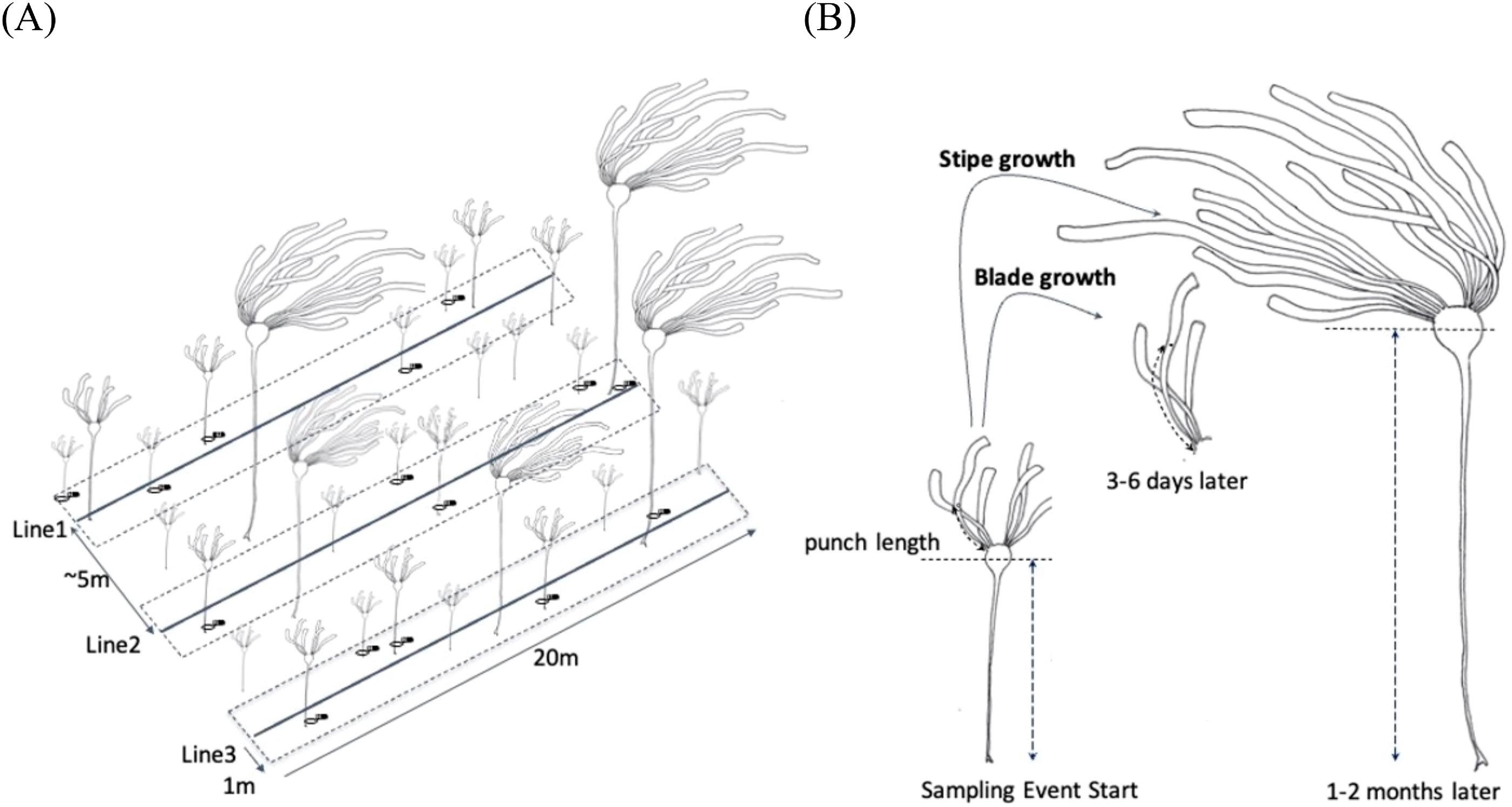
Sites were selected to represent common conditions (e.g., depth, exposure, substrate type) of N. luetkeana rocky reef habitat in this region. Three kelp sites adjacent to Calvert and Triquet Island on the Central Coast of British Columbia (BC), Canada were established: North (North Beach), Second (Second Beach), and Manley (Fig. 1). Substrate types ranged from boulder (North) to cobble and bedrock (Manley and Second), with some sand encroachment (Second). Sites were either long-established (Manley) or recently re-established (North and Second) following sea otter recolonization between 2013 and 2014 (Burt et al. 2018). The survey design consisted of three 20 m permanent lead-weighted transects 5 m apart and parallel to one another along the 2–4 m MLLW (Mean Lower Low Water) depth contour (Fig. 2).
Fig. 1.
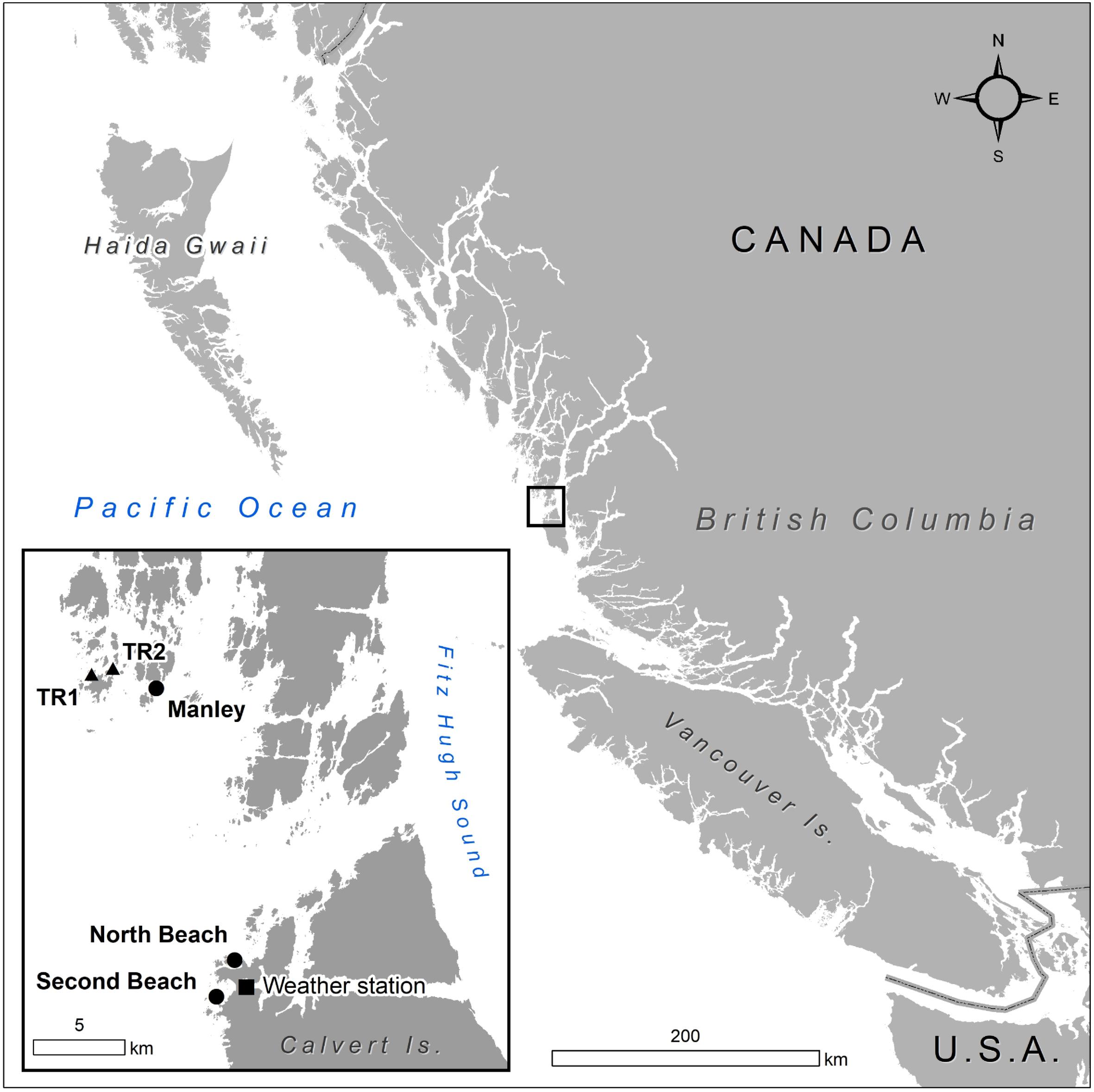
Fig. 2.
Kelp surveys, using SCUBA occurred seasonally, 4–6 times per year (sampling events) from 2016 to 2018 (May to November), and twice in 2019 (January and July). These surveys are a component of the Hakai Institute Kelp Monitoring Program (Pontier et al. 2022). The timing of sampling events was based on prior observations of recruitment and growth of N. luetkeana at these sites. Recruits of N. luetkeana (sporophyte stage) were observed in early April, and plants reached 1 m stipe length by May. Most individuals in the population persisted until November, but rarely into the following year.
During each sampling event, we haphazardly selected up to 15 individuals of N. luetkeana >=1 m stipe length within 1 m of the permanent transect lines at each site (Fig. 2A). We tagged individual thalli using numbered flagging tape, which was later removed at the end of each sampling event. We did not keep track of tagged individuals over the course of the year; resampling of individuals is likely, especially when fewer than 15 individuals were found. In this instance, all individuals were tagged and recorded. Depth was recorded at each 5 m interval once and corrected for tidal height, thereafter individual kelp holdfasts were assigned to the closest known 5 m interval depth. Bulb depth was calculated as stipe length subtracted from holdfast depth (such that positive numbers are bulbs below water and negative numbers are bulbs trailing on the surface).
Blade and stipe measurements
Blade
For each tagged individual and at the start of each sampling event, we selected one of the two distal blades and measured its length as the distance from the blade attachment point against the pneumatocyst to the end of the blade (Supplementary Materials, Table S1: Initial Blade Length). We also punched a single hole through the blade, at a distance of one third its length (Fig. 2A). We standardized blade punching using this method (as opposed to using a fixed distance from the attachment point) because 95% of the total blade growth occurs in the proximal third to half of the blade and is predominantly lengthwise (Kain 1987). After 3–6 days (Supplementary Materials, Table S1, Fig. 2B) we measured the new distance of the punch mark as well as the full blade length. Daily blade growth was calculated as the difference between the initial and final punch mark measurements, divided by the number of days of growth.
Stipe
Stipe length was also measured at the start of each sampling event as the distance from the holdfast to halfway up the pneumatocyst (Supplementary Materials, Table S1: Initial Stipe Length), and re-measured at the start of the following sampling event (Fig. 2B, ∼1–2 months, with some re-measurements after 16–91 days due to logistical challenges). Daily stipe growth was calculated as the difference between initial and final measurements of stipe length, standardized by the number of days of growth.
Isotopes
Blades were collected after each final measurement and a 5 cm × 5 cm section was cut out 10 cm above the pneumatocyst. Samples were gently cleaned with deionized water, oven dried at 60 °C for at least 24 h or until dry and grinded before being packed in tin capsules for isotopic measurement using continuous-flow Isotope-Ratio Mass Spectrometry at UC Davis. δ15N signatures were calculated relative to international standards (in air).
Abiotic environmental factors
As explanatory variables (Supplementary Materials, Table S1), water temperature and nutrients were measured in situ at each site, and surface light availability was derived from the closest weather station. We interpolated and/or extrapolated missing temperature (Supplementary Material, Fig. S1) and nutrient data using data from adjacent sites with similar average depths and exposure (Fig. 1).
Temperature
At each site, water temperature was measured at 15 min intervals using HOBO loggers (Onset HOBO TidbiT v2 and Pendant) deployed at depths of 2.5–3.1 m MLLW. For each sampling event, mean daily temperature metrics were calculated for the time period associated with blade growth (3–6 days), and time period associated with stipe growth (1–2 months). Extrapolation based on adjacent sites was done for missing data (details in Supplementary Materials and Methods, Fig. S1).
Nutrients
Water samples were collected at depths of 0, 5 and 10 m (except for Second where only 0 and 5 m samples were collected) and within 100 m of surveyed sites bimonthly, monthly or as feasible during the primary growing season (May—September). Water samples were frozen at the Calvert Island Observatory and later nitrate and nitrite concentrations (NO2− and NO3−) were analyzed at the University of British Columbia, on a Lachat QuikChem 8500 Series 2 Flow Injection Analysis System (Smith and Bogren 2003). During the timeframe of these surveys, few nutrient samples were collected at Manley. Additional nutrient concentrations were extrapolated for the Manley site by averaging the values at two adjacent sites (TR1 and TR2) (Fig. 1). Mean monthly nitrate-nitrite concentrations per site were calculated by averaging NO3−+NO2− concentrations (µM/L) across all water depths. All sites are located on exposed reefs where water mixing due to wave action is common in the top 5–10 m.
Light
Light concentrations were obtained from photosynthetically active radiation (PAR) collected at 5 min intervals from a Quantum PAR Sensor (PQS1) located on a weather station on the northwest side of Calvert Island Hakai Institute Ecological Observatory (Fig. 1). We used the same values for all sites (Supplementary Materials, Table S1), located approximately 1.9 km (North), 1.7 km (Second) and 17.3 km (Manley) away. Daily Light Integral (DLI: mol/m2/day) was calculated to provide an integrated value of total daily dosage of light (light availability) and incident photon flux density, which is strongly related to plant growth (Poorter et al. 2019). For each sampling event, mean daily light integral metrics were calculated for the time period associated with blade growth (3–6 days), and the time period associated with stipe growth (1–2 months).
Statistical analysis
Model structures
To explore the expected nonlinear relationships between growth rates, abiotic factors, initial lengths, and annual phenology three Bayesian Regression Models (BRMs) were constructed for blade growth (models 1 and 2) and stipe growth (model 3) based on a priori understanding of the ecological roles of these factors on kelp productivity (Supplementary Materials, Table S1). Model 1 included temperature, nutrients, light availability (DLI), depth, day of year (DOY), and initial blade length as predictors of blade growth (Supplementary Materials, Table S1) for the primary growing season of N. luetkeana (May to September, 2016–2019). Model 2 included the same predictors, but data from all seasons (November 2016, 2018, and January 2019) was included, and nutrient concentrations as a predictor were excluded (nutrient data was not available outside of the primary growing season). Model 3 used the same suite of predictors to examine stipe growth, except initial stipe length was used as a predictor (instead of blade length). The dataset included the primary growing season (May to September, 2016–2019), as well as three of the sampling events for which stipe growth was measured between late summer and early November (September 2016, August 2017 and August 2018). Nutrient estimates for these three sampling events are based on August and/or September data only.
Thin-plate splines were fit to model relationships with temperature, nutrients, light, depth, and blade or stipe length, whereas cyclic cubic splines modeled growth rates by DOY. For all models, we limited the dimension for smoothers (K) to a maximum of 4 to simplify the interpretation of results and avoid overfitting (Lopez et al. 2017). Models included a random effect of site, with an offset for the time allowed for growth (log(time)). Since samples collected for each sampling event within sites were not independent, we considered each model with and without compound symmetry structure (COSY). Accounting for independence did not influence model results, so COSY was not included in the final model results and predictions (Supplementary Materials, Figs. S2, S3, S4). All models used a Gamma likelihood distribution and a log link, and models ran using Hamiltonian Monte Carlo (HMC) fit, using flat priors.
Models and predictor performance
All three models were used to estimate how individual predictors affected change in growth and the maximum and minimum amount of growth (upper and lower bounds to growth) (Figs. 7 and 8, Table 1). For each model, we estimated Bayes R-squared values (a metric of variance explained) as well as an approximation to leave-one-out cross validation (LOO, a metric of out of sample predictive accuracy). We estimated these metrics with and without the compound symmetry structure using Stan via the R package brms (Bürkner 2017) (Supplementary Materials, Table S4 and Table 2, respectively).
Table 1.
| (A) | |||||
|---|---|---|---|---|---|
| Predictor variable | Value of predictor for min growth | Value of predictor for max growth | Value of predictor for max rate of (+ or –) change in growth | Whole-unit change in predictor (×) near max rate of change in growth | Related % change in growth per whole-unit change in predictor |
| Temperature (°C) | 13.2 | 10.0* | 11.9 (−) 14.1 (+) | 11–12 (1 °C) 13.5–14.5 (1 °C) | 23% loss (−1.1 cm/day) 25% gain (1.4 cm/day) |
| 14.7* | 8.9 | 11.6 (−) | 11–12 (1 °C) | 23% loss (−1.0 cm/day) | |
| Nutrient (µM/L) | 0.1* | 13.4* | 0.1 (+) | 0.1–1.1 (1 µM/L) | 34% gain (1.4 cm/day) |
| NA | NA | NA | NA | NA | |
| DLI (mol/m2/day) | 17.1* | 35.9 | 19.5 (+) 43.7 (−) | 19–29 (10 mol/m2/day) 43–53 (10 mol/m2/day) | 23% gain (1.0 cm/day) 23% loss (−0.8 cm/day) |
| 3.7* | 28.8 | 17.1 (+) 39.1 (−) | 17–27 (10 mol/m2/day) 39–49 (10 mol/m2/day) | 27% gain (1.1 cm/day) 21% loss (−0.7 cm/day) | |
| Bulb depth (m) | −5.5* | 3.3* | −4.3 (+) | −5 to −4 (1 m) | 10% gain (0.4 cm/day) |
| −5.9* | 3.3* | −5.4 (+) | −6 to −5 (1 m) | 1% gain (0.04 cm/day) | |
| Initial length (cm) | 8* | 268* | 62 (+) | 62–72 (10 cm) | 10% gain (0.4 cm/day) |
| 8* | 326* | 268 (+) | 255–265 (10 cm) | 4% gain (0.4 cm/day) | |
| Day of year (m., month) | 233 (Aug21) | 163 (Jun12) | 142 (+) 184 (−) | 135*–165 (1 m., spring) 165–195 (1 m., summer) | 30% gain (1.5 cm/day) 25% loss (−1.0 cm/day) |
| 317 (Nov13) | 194 (Jul13) | 141 (+) 233 (−) | 135*–165 (1 m., spring) 245–175 (1 m., fall) | 2% gain (0.1 cm/day) 1% loss (−0.1 cm/day) | |
| Note: day 142 (May 22), day 184 (Jul 3), day 141 (May 21), day 233 (Aug 21). | |||||
| (B) | |||||
| Temperature (°C) | 12.7 | 10.3* | 10.3 (−) 14 (+) | 10.3–11.3 (1 °C) 13.5 –14.5 (1 °C) | 64% loss (−2.5 cm/day) 16% gain (0.5 cm/day) |
| Nutrient (µM/L) | 0.1* | 1.22 | 0.2 | 0.2–1.2 (1 µM/L) | 71% gain (2.4 cm/day) |
| DLI (mol/m2/day) | 13.3* | 41.3* | 13.3* | 14–24 (10 mol/m2/day) | 31% gain (0.7 cm/day) |
| Bulb depth (m) | −4.6* | 3.3* | 3.0 | 2 to 3 (1 m) | 22% gain (1.9 cm/day) |
| Initial length (cm) | 707* | 293 | 94 519(−) | 94–104 (10 cm) 519–529 (10 cm) | 2% gain (0.03 cm/day) 3% loss (−0.1 cm/day) |
| Day of year (m., month) | 223 (Aug11) | 161 (Jun10) | 141(+) 183(−) | 135*–165 (1 m., spring) 165–195 (1 m., summer) | 21% gain (0.7 cm/day) 42% loss (−1.0 cm/day) |
Note: *indicates lowest/highest recorded measurements.
Table 2.
| Model | Factor removed | LOO | R2 |
|---|---|---|---|
| Blade model 1 (primary growing season) | NA (full model) | 0.499 | 0.66 |
| Temperature | 0 | 0.62 | |
| Nutrients | 0 | 0.62 | |
| DLI | 0.116 | 0.65 | |
| Bulb depth | 0.286 | 0.66 | |
| Initial blade length | 0.098 | 0.58 | |
| Blade model 2 (full time series) | NA (full model) | 0.916 | 0.61 |
| Temperature | 0.022 | 0.59 | |
| DLI | 0 | 0.59 | |
| Bulb depth | 0 | 0.61 | |
| Initial blade length | 0.062 | 0.47 | |
| Stipe model (primary growing season) | NA (full model) | 0.727 | 0.69 |
| Temperature | 0 | 0.71 | |
| Nutrient | 0.110 | 0.68 | |
| DLI | 0 | 0.70 | |
| Bulb depth | 0 | 0.68 | |
| Initial stipe length | 0.163 | 0.69 |
Note: For results with compound symmetry covariance structure (COSY), see supplement.
In addition to models including covariates, we also constructed models that included year, site, and their interaction to assess and quantify interannual and spatial variation in growth dynamics during the study period. We conducted all statistical analyses in R version 4.1.1.
Results
Changes in environmental conditions co-occurred with changes in growth rates over the primary growing season. Though optimal growth conditions were often present in the spring months (May and June), environmental drivers fluctuated independently, allowing significant and variable growth rates, throughout the primary growing season. Optimal growth of N. luetkeana (∼13–14 cm/day for blades and stipes) occurred within a narrow range of local environmental conditions. Maximum blade and stipe growth occurred at lower water temperatures (around 10 °C), above 1 µM/L nitrate concentration, and at moderate light levels (daily light integral or DLI 20–40 mol/m2/day). Blade and stipe growth decreased rapidly at temperatures >10 °C, below 1 µm/L nitrate, and surface light reduced blade growth at low and high levels (<20 and >40 mol/m2/day).
Trends in blade and stipe growth rates
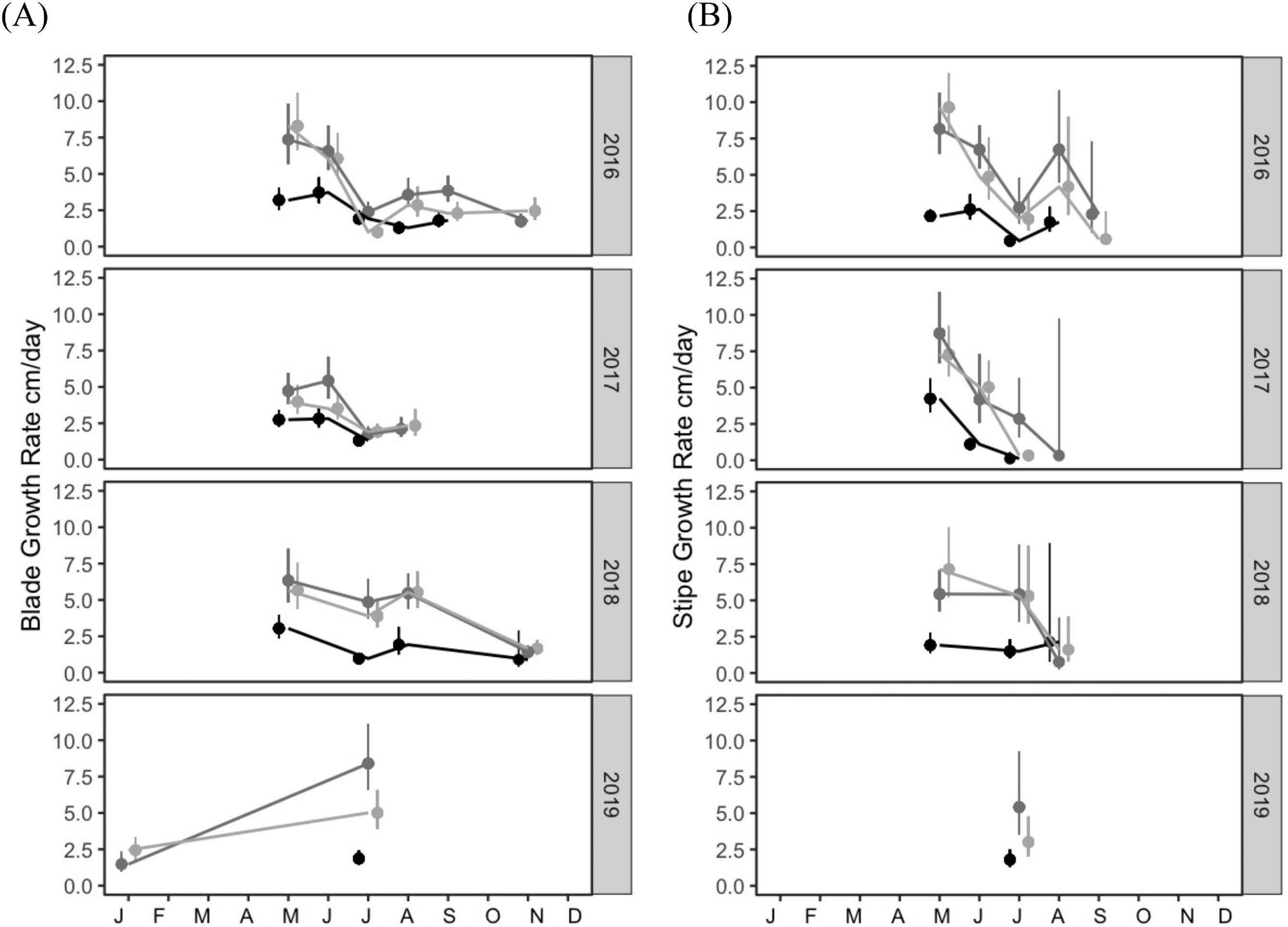
N. luetkeana blade growth (N = 601 individuals) and stipe growth (N = 377 individuals) exhibited similar overall maxima but varied independently across sites, seasons and years (Table S2; Fig. 3). Blade and stipe growth for individual plants ranged from 0 to 13.72 cm/day for blades and 0 to 12.96 cm/day for stipes, with higher average growth rates generally observed in May for stipe and throughout the primary growing season (May through September) for blades (Fig. 3). Across all sites and years, mean growth rates per sampling event ranged from 0.83 ± 0.20 cm/day to 8.25 ± 0.78 cm/day for blades and 0.23 ± 0.15 cm/day to 9.31 ± 0.75 cm/day for stipes (Fig. 3).
Fig. 3.
Year, site and their interaction were all strongly associated with blade growth (LOO = 0.953) and explained a greater proportion of total variation (R2 = 0.63) than alternative models (LOO = <0.01 and R2 < 0.6). Stipe growth was most strongly associated with interannual variability (LOO = 0.664 for year only model) rather than full model (LOO = 0.298 including year, site and their interaction) though both models explained an equal portion of the variance (R2 = 0.66 for both).
Blade growth had the lowest averages throughout the year in 2017 compared to 2016 and 2018 (2.85 vs 3.32, 3.68 cm/day, respectively). Variation between sites was also observed; on average, Manley had lower blade and stipe growth rates than both North and Second, where rates overlapped (Fig. 3). Stipe growth was highest in Springs of 2016 and 2017, and lower in 2018 (May averages: 6.20, 6.22 and 4.10 cm/day, respectively) but overall, not as high through Summers of 2016 and 2017 compared to 2018 and 2019 (July averages: 1.4 and 1.05 in 2016 and 2017 vs 3.05 and 2.87 cm/day in 2018 and 2019, respectively).
Isotope analysis
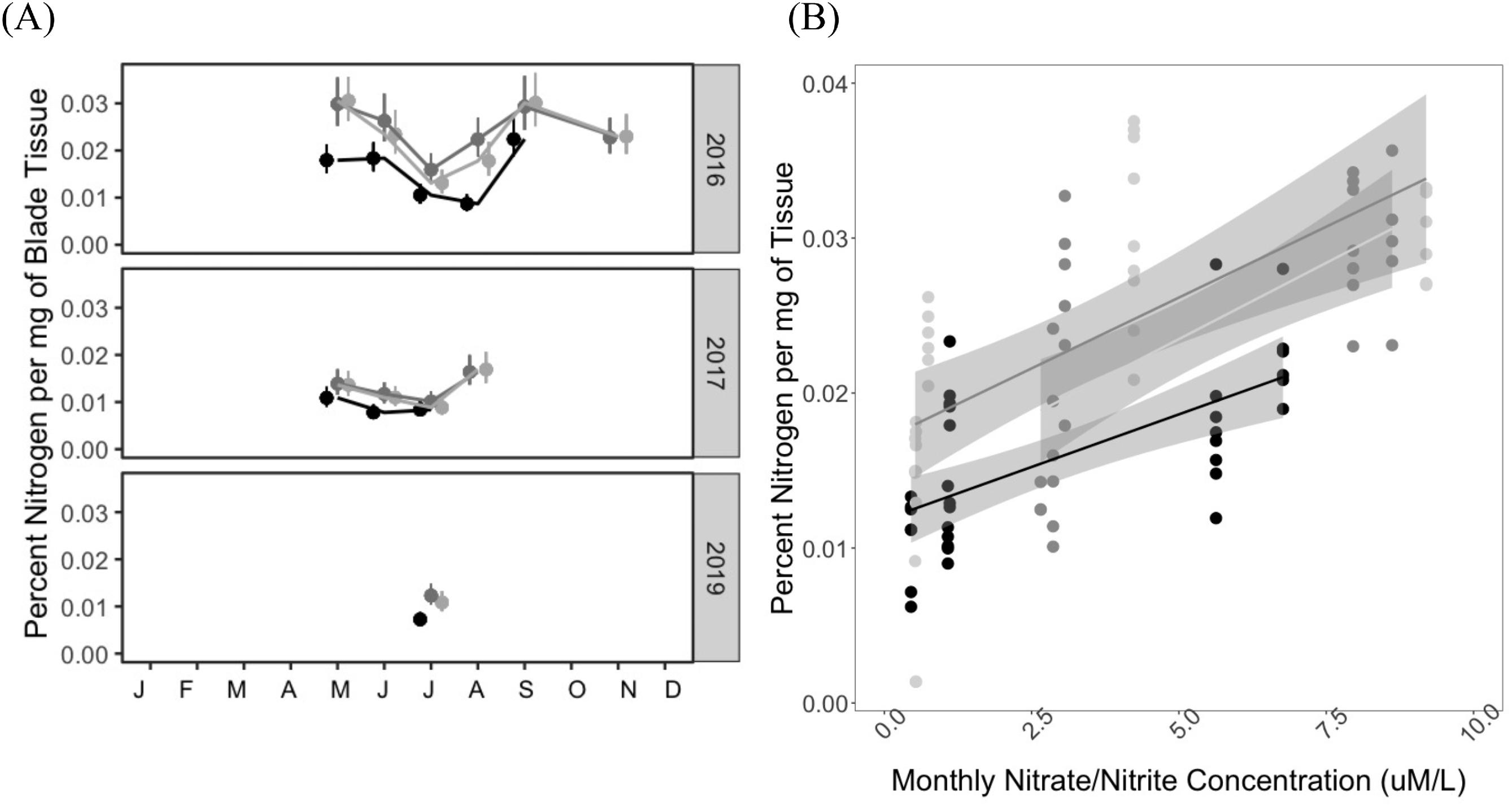
Mean percentage of nitrogen per gram of blade tissue also varied across seasons, with the greatest percentages across individuals in May (2.83%–3.75%) and September (2.80%–3.56%) relative to July (1.3%–2.4%) (Fig. 4A). Site differences were also observed, with Manley consistently lower on average (1.3%, 0.5%–2.8%) than North and Second (1.9%, 0.6%–3.6% and 1.9%, 0.1–3.7, respectively). Percent tissue nitrogen was also strongly correlated with nitrogen concentrations obtained from water samples (R2 = 0.42 Manley, R2 = 0.45 North and Second, p < 0.001 for all sites, Fig. 4B).
Fig. 4.
Empirical trends in abiotic environmental factors
Mean daily water temperature, nutrient (NO2− and NO3−), and daily light integral (DLI) of surface light (hereafter referred to as temperature, nutrients, and light, respectively) exhibited strong seasonal effects, and smaller differences across sites, and years, with the highest variability over the summer months (Table S2; Fig. 5).
Fig. 5.
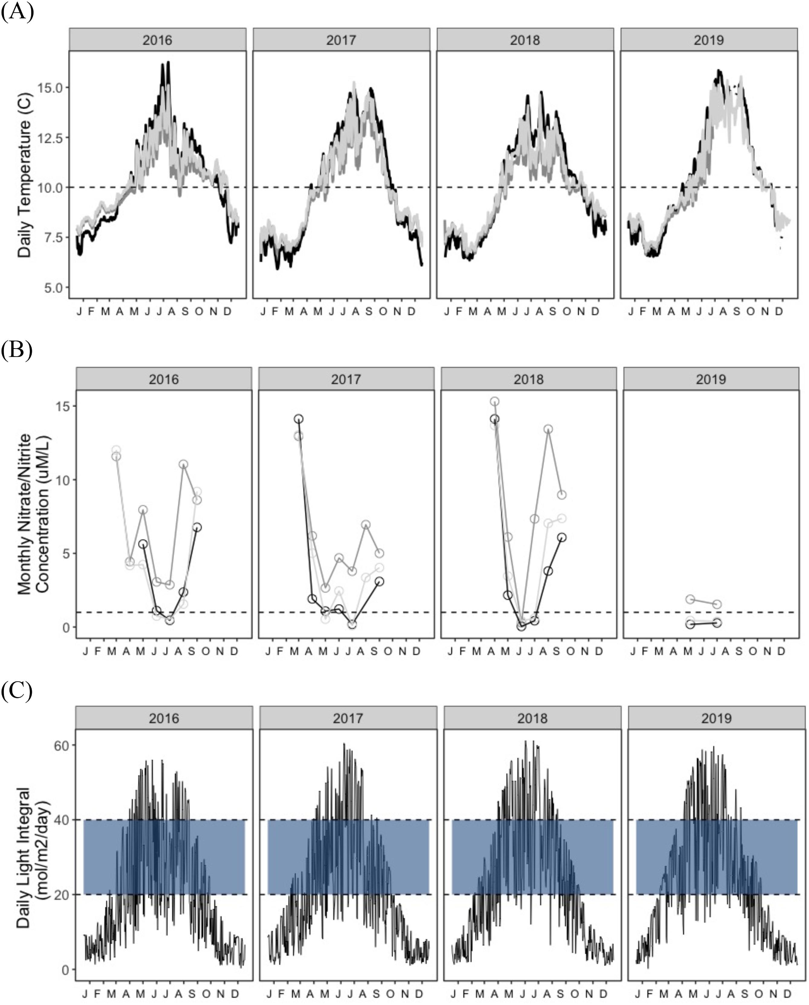
Temperature trends
Temperature was lowest and least variable in winter and spring (range: 5.9–10.6 °C and 6.0 °C–12.3 °C, respectively) and highest and more variable in summer and fall (range: 9.4–16.3 °C and 8.0–15.5 °C, respectively) (Table S2; Fig. 5A), with higher peaks in 2016 and 2019 summers, and fall of 2017. Manley experienced warmer summer and colder winter temperatures compared to the other sites (Table 2). North consistently experienced the least variability and lowest overall summer temperatures (Table S2).
Nutrient trends
Nutrients (NO2− and NO3−) were greatest and, more variable over the spring (range: 0.2–15.3 µM/L) and summer (range: 0.04–13.4 µM/L) relative the fall (range: 3.09–9.2 µM/L). Steepest and earliest declines (to below 1 uM) occurred in 2017 and 2018 (Fig. 5B). North had higher relative nutrient concentrations (range: 0.29–13.4 µM/L) and were on average 2.93–3.48 µM/L higher than Second and Manley (0.11–9.20 and 0.04–6.77 µM/L, respectively), across the primary growing season.
Light trends
Mean daily light integral (DLI) varied seasonally, with the lowest and least variable values in winter and fall (ranges: 0.2–24.5 mol/m2/day and 1.1–40.5 mol/m2/day, respectively) and the highest and most variable values in spring and summer (ranges: 2.47–58.8 mol/m2/day and 6.52–61.1 mol mol/m2/day, respectively) (Table S2, Fig. 5C). The seasonal light regime was consistent across years (Fig. 5C).
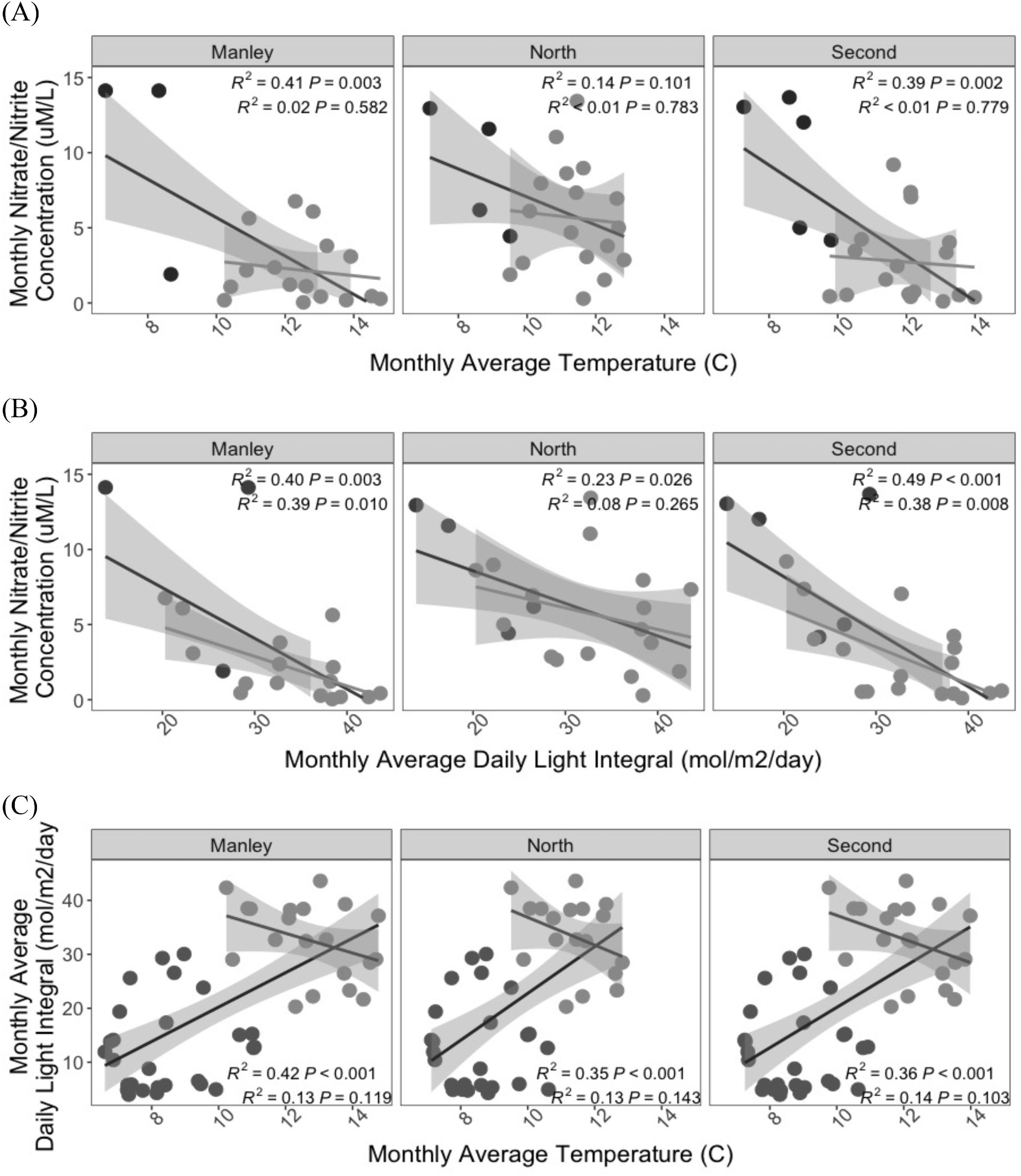
Environmental correlations
Though temperature, nutrient and DLI trends were correlated across sites for the full year time series (Fig. 6, p < 0.05, except for nutrient and temperature at North), these relationships were not observed across the primary growing season (Fig. 6, p > 0.05, except for nutrient and DLI at Manley and Second). Monthly temperature and DLI averages were negatively correlated with nutrients for both the full time series and the primary growing season (Figs. 6A and 6B) while the relationship between temperature and DLI changed from positive (full time series) to negative (primary growing season only) (Fig. 6C).
Fig. 6.
Predictors of blade and stipe growth rates
All factors (temperature, nutrients, light, initial blade/stipe length and bulb depth) were related to blade and stipe growth, with strong evidence to support the full model over alternative models that excluded each factor based on LOO relative model weights (Table 2). The full models also explained a greater proportion of total variation in blade and stipe growth, respectively, relative to alternative models based on R-squared values (Table 2).
Temperature
Across the full time series, blade growth (model 1) exhibited a unimodal relationship with temperature (Fig. 7A) while the primary growing season models (blade growth model 2 and stipe growth model 1) only captured the downward portion of the relationship with a slight increase at extreme temperatures for which growth data was limited (Figs. 7A–7B, Tables 1A–1B). Maximum blade growth was predicted at the lowest recorded growth season temperatures (8.0–12 °C, with a peak at 8.9 °C across the full year (model 1) and at 10.0 °C during the primary growing season (model 2; Fig. 7A, Table 1A). Maximum stipe growth was also predicted at the lowest recorded temperatures (10.3 °C) over the primary growing season, with the greatest deceleration in growth following this peak and the lowest stipe growth at 12.7 °C (model 3; Fig. 7B, Table 1B).
Fig. 7.
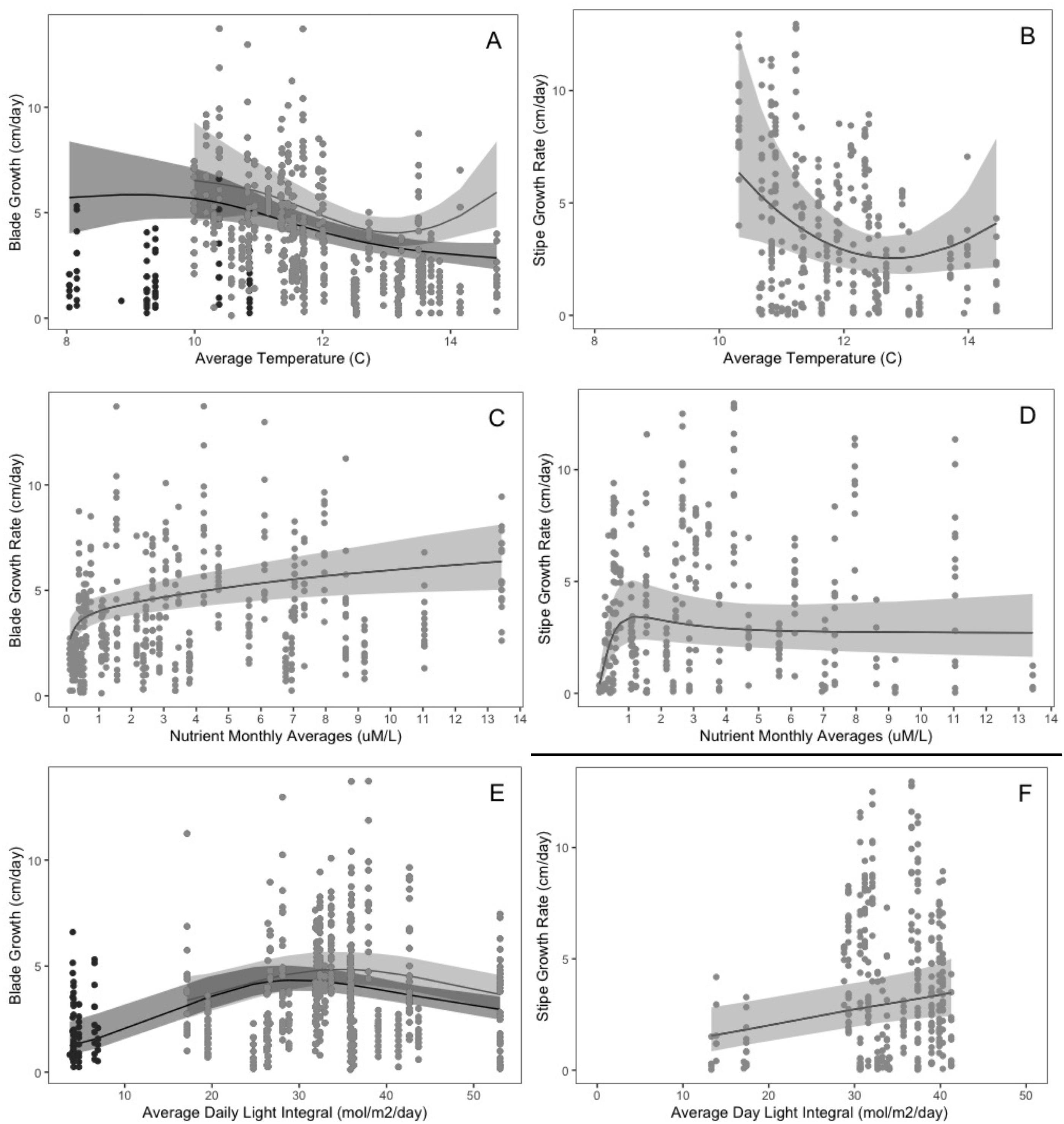
Nutrients
Blade growth and stipe growth showed nonlinear, positive relationships with nutrients (Fig. 7C–7D and Tables 1A–1B). Blade and stipe growth increased rapidly with nutrient concentrations of 0.1 to 1 µM/L, with the greatest acceleration in growth at 0.1 µM/L for blade growth and at 0.2 µM/L for stipe growth (Figs. 7C–7D and Tables 1A–1B). Blade growth rates slowed following the initial exponential trends, peaking at the highest recorded nutrient concentration (13.4 µM/L) while stipe growth peaked at concentration of 1.22 µM/L before plateauing.
Light
Blade growth displayed a hump-shaped relationship with daily light integral (DLI) (Fig. 7E and Table 1A), while stipe growth exhibited a positive, linear relationship with DLI (Fig. 7F and Table 1B). Blade growth peaked at 28.8–35.9 mol/m2/day, and declined to a minimum at the lowest recorded DLI (3.7 mol/m2/day) for the full time series and at the highest recorded DLI (17.1 mol/m2/day) for the primary growing season (Fig. 7E and Table 1A). Minimum stipe growth occurred at the lowest recorded DLI for the primary growing season (13.3 mol/m2/day) and increased linearly with DLI until its peak growth rate at the maximum recorded light level (41.3 mol/m2/day) (Fig. 7F and Table 1B).
Bulb depth
Blade growth exhibited a near-linear, weakly positive relationship with bulb depth, while stipe growth was nonlinear and strongly positive with bulb depth (Figs. 8A–8B and Tables 1A–1B). Blade and stipe growth were both greatest for the deepest recorded bulb depths (3.3 and 2 m respectively). Both growth rates continued to decrease as stipe length increased on the water surface (negative bulb depths indicate that the portion of stipe trailing on surface is above 0 chart datum). The lowest growth rates were predicted for the smallest recorded values (−5.5 m blade model 1, –5.9 m blade model 2 and –4.6 m stipe model), though the relationship was much weaker for blade growth. Stipe growth increased at an accelerated rate with bulb depth, with a maximum rate of change at 1.2 m below surface (Fig. 8B andTable 1B).
Fig. 8.
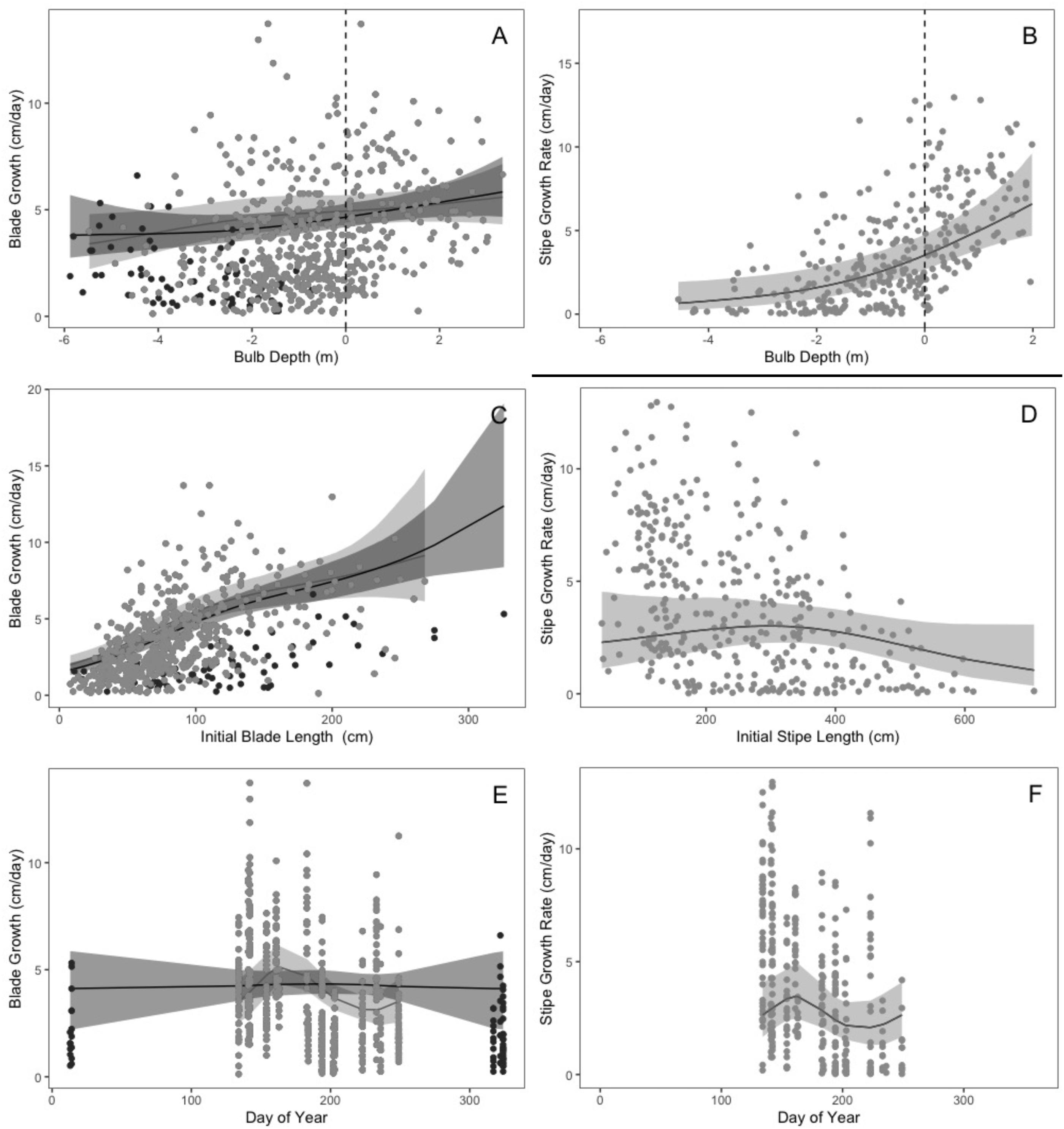
Initial blade/stipe length
Blade growth was positively and nonlinearly related with initial blade length, while stipe growth showed a hump-shaped relationship with initial stipe length (Figs. 8C–8D and Tables 1A–1B). Blade growth was lowest for the shortest measured blades (8 cm). Blade growth exhibited a near-linear increase with longer blade lengths from 8 to 100 cm, after which the rate of increase slowed with the highest blade growth observed for the longest blades (268–326 cm) (Fig. 8C and Table 1A). However, few blades longer than 200 cm were surveyed, increasing the 95% prediction intervals above 200 cm. Stipe growth increased with initial stipe length from 39 to 293 cm, where it peaked and thereafter decreased to a minimum at 707 cm, with the caveat that very few stipes longer than 580 cm and shorter than 100 cm were surveyed (Fig. 8D and Table 1B).
Day of year
Blade and stipe growth were cyclically related with day of year except for a weak, nonlinear relationship with day of year for the full time series model (model 2; Figs. 8E–8F and Tables 1A–1B). Blade growth peaked at the beginning of summer (day 163/June 12th) over the primary growing season and declined to its lowest value in late summer (day 233/August 21st) (Fig. 8E and Table 1A). Similarly, stipe growth peaked at the beginning of summer (day 161/June 10th) over the primary growing season and declined to its lowest value in mid to late summer (day 223/August 11th) (Fig. 8F and Table 1B).
Discussion
Growth dynamics of marine macroalgae are integral properties of primary productivity and provisioning of habitat. Growth rates also have the capacity to serve as indicators of marine climate stress if the magnitude and directionality of their responses to environmental conditions can be quantified and interpreted. We conducted over 600 measurements of individual blade and stipe growth at three sites on the Central Coast of British Columbia. These spanned four years, representing substantial spatial as well as intra- and interannual variation in environmental conditions in this region. We found that individual bull kelps exhibited considerable spatial and temporal variation in growth rates (ranges: 0–13.72 cm/day for blade and 0–12.96 cm/day for stipe). These results highlight the potential for high productivity in this species, as well as its sensitivity to key environmental conditions as predicted for annual autotrophs subject to environmental fluctuations (Morris et al. 2008; Compagnoni et al. 2021). Specifically, growth rates exhibited significant and nonlinear responses to changes in temperature, nutrients, and light. In this system, nutrient concentrations and temperature were decoupled during the primary growing season (May to September) of N. luetkeana, demonstrating that the response and sensitivity of biological indicators requires simultaneous in-situ measurements of local environmental conditions. Overall, our results demonstrate that shifts in growth rates, one metric of kelp productivity, will be valuable metrics for the management of this foundational species and may be used as bioindicators of change in marine research, planning and conservation.
Spatiotemporal variability in N. luetkeana growth rates and environmental factors
Through this study, growth rates varied seasonally as well as across years and among sites (Fig. 3, Figs. 8E/F, and Supplementary Materials Table S2). Seasonal patterns in growth rates reflect this kelp’s life history strategy to grow quickly in the spring (associated with an increase in daylight period, Vadas 1972) and irregularly throughout the summer (associated with local conditions, Foreman 1984), before annual dislodgement in the fall and winter. These variable patterns of growth in response to environmental conditions were also observed across sites. For example, individuals at the Manley site, which exhibited lower growth rates relative to the other two sites, were exposed to both higher peak temperatures as well as earlier onset and prolonged periods of low nutrient concentrations in the summer (Fig. 5) which was reflected in low % nitrogen content in blade tissues in comparison with the other sites (Fig. 4A). We observed a similar decrease in stipe and blade growth as well as % nitrogen content in blades across sites following the early season low nutrient onset in 2017 in comparison with 2016 and 2018 seasonal trends (Fig. 3 and Supplementary Materials Table S2). In the context of climate-related stress, this strong response of N. luetkeana to seasonal, site-level, and interannual changes in environmental conditions likely predisposes this species to magnified negative effects associated with localized climate fluctuations.
Environmental conditions also varied across sites, seasons and years, but only co-varied consistently when pooled over the full year which did not reflect trends over the primary growing season of N. luetkeana (May to September). Nutrient concentrations decreased with increasing light availability, a pattern that was consistent within the primary growing season and across the full year (Fig. 6B). By contrast, temperature decreased with light availability during the primary growing season (though not significantly), but increased with light across the full year (Fig. 6C). These differing seasonal trends for nutrients and temperatures underpin their temporal decoupling. Nutrient and temperature correlations were strongly negative throughout the full time series, but weakened considerably over the primary growing season of kelp (Fig. 6A) which likely influenced its growth patterns seasonally.
N. luetkeana growth rate response to specific factors
Temperature effects
Growth rates slowed by 16% to 64% as temperature increased by a degree from their observed thermal optimum (∼ 9 °C–11 °C, Figs. 7A/B and Table 1). Growth rates also slowed dramatically above 12 °C. With summer sea surface temperature now exceeding 12 °C for a large portion of the primary growing season, growth dynamics in this region are likely already experiencing thermal limitations in the summer. These findings reflect other studies in the Salish Sea (Wheeler et al. 1984; Supratya et al. 2020; Fales et al. 2023) and northern California (Rogers-Bennett and Catton 2019) where growth is negatively impacted by increasing temperature. However, our in-situ results are on the lower end of previously described thermal optimum from laboratory experiments. Supratya et al. (2020) indicated that N. luetkeana collected from the Strait of Georgia (BC) showed peak growth at 11.9 °C, with substantial declines thereafter. Similarly, Fales et al. (2023) in Washington State, found a higher temperature optimum between 12 °C and 15 °C. Temperatures required for optimal growth of N. luetkeana overlapped with ranges observed for other dominant canopy-forming kelp in this region, including the perennial M. pyrifera which can be a competitor for space in this particular region of the coast. Temperatures resulting in negative effects on M. pyrifera were slightly higher: 12–13 °C on the Central Coast of BC (Krumhansl et al. 2017), and 16°C–20 °C for M. pyrifera in southeastern Alaska (Umanzor et al. 2021). Overall, temperature-growth rate relationships suggest that projected climate-driven increases in mean and extreme temperatures could substantially decrease growth of canopy-forming kelps such as N. luetkeana in many areas of the northeastern Pacific Ocean.
Nutrient effects
While N. luetkeana showed gradual negative responses to changing temperatures, nutrient thresholds were more pronounced and acute. With respect to nutrient limitation, growth remained unaffected until water nitrate concentrations fell below approximately 1 µM/L which generally occurred every summer, though not across all sites, and varied in its onset (April to August) and duration (up to several months) across years (Fig. 5B). Nutrient concentrations slowed growth by 34% to 71% as they dropped to the lowest observed value of 0.1 µM/L (Figs. 7C/D and Table 1). This relationship demonstrates a strong positive response strategy to pulses of nitrate, but also, a negative response to prolonged periods of nitrate-deplete conditions. Growth was episodically nutrient limited (dropped below 1 µM/L) over the summer months (particularly June and July) and as early as spring (April and May). This aligns with laboratory studies where nitrate concentrations below 2 µM/L limited photosynthetic performance and nitrate tissue content in N. luetkeana (Wheeler et al. 1984; Rosell and Srivastava 1985), though recent work by Fales et al. (2023) found no effect in growth with nitrate concentrations below 0.59–1.04 µM/L, indicating that this threshold may be lower than previously reported. Tissue nitrate content also tracked water nitrate concentration in our study (Fig. 4), building on evidence that N. luetkeana can readily uptake (Ahn et al. 1998) and assimilate nitrate when available in sufficient quantities (Wheeler et al. 1984). Moreover, N. luetkeana only stores nitrate for short time periods (15–30 days; Gerard 1982; Brown et al. 1997) if at all (Wheeler and North 1980) making it particularly sensitive to prolonged localized nitrate-depletion. The observed nutrient-growth rate relationships emphasize the importance and rapid response of N. luetkeana growth to changes in nutrient conditions, especially at low concentrations.
Temperature-nutrient decoupling
While both temperature and nutrient had strong and rapid nonlinear effects on growth rates, they also exhibited seasonal and periodic decoupling. Thus, each episodically imposed independent limitations on growth as temperature and nutrients were not correlated within the primary growing season (May to September) in this region (Figs. 5 and 6). This contrasts with other regions in the northeastern Pacific including southern California (Jackson 1977; Zimmerman and Kremer 1984; Dayton et al. 1999) where nutrient or temperature limitation occur tandem and track one-another closely across seasons and years (Parnell et al. 2010; García-Reyes et al. 2014; Cavole et al. 2016; Jacox et al. 2018). As a result of decoupling in this study, temporal offsets gave rise to multiple periods throughout the primary growing season, and through the full year, where different abiotic conditions placed limits on kelp growth. For example, periods of favorable, high nutrients were observed with high, unfavorable temperatures, while periods of unfavorable, low nutrients were observed with favorable temperatures. Furthermore, at some times of the year, both temperature and nutrients conditions existed in their unfavorable or favorable range. These temporal trade-offs in growth regulation emphasize that multiple factors are responsible for changes in growth rate indicators, requiring local knowledge of the system to interpret the mechanisms regulating population dynamics.
Light, depth, and morphological effects
DLI, a measure of total daily light dosage and incident photon flux density, values remained sufficiently high throughout the primary growing season (May to September) to support high blade growth (Fig. 7E and Fig. 8A). Stipe growth was more influenced by periods of sustained low DLI over several weeks (i.e., 31% change in growth in association with 10 umol/m2/s change in average DLI over the primary growing season; Fig. 7F and Table 1B). Although DLI was highly variable across days (particularly over the primary growing season), the effects of single days of low or high irradiance did not impede blade growth or stipe growth over periods of a few days to weeks. Other research also suggests that N. luetkeana is well-adapted to daily and seasonal fluctuations in PAR availability (Foreman 1984; Wheeler et al. 1984; Koehl and Alberte 1988) and photoperiod (Dickson and Waaland 1985; Maxell and Miller 1996). Nevertheless, blades were still sensitive to sustained exposure to light, with an average 21%–23% decline in blade growth associated with an increase of 10 mol/m2/day above the DLI optimal range (29–36 mol/m2/day). We anecdotally observed blade and bulb senescence at the water surface in peak summer (with periods of high light and temperature). This was also illustrated in a lab experiment where sustained irradiance above 1000 umol/m2/s led to 40% declines in photosynthetic efficiency of this species (Poulson et al. 2011). These relationships highlight again the reactive nature of growth in this canopy forming species to extreme events and the potential compounding effects of light with other drivers such as warming at the water surface.
Surprisingly, light attenuation with depth in the water column was not strongly related to growth. Instead, we observed a steep increase in stipe growth with bulb depth and a decrease in stipe growth with stipe length, reflecting a shift in energy allocation from stipe elongation to sori production as the stipe reaches the surface (Foreman 1970). Similarly, blade growth did not decrease with bulb depth, building on evidence that blade elongation rates are consistent throughout the kelp’s ascension to the surface and through sori production, where sori are produced and shed (for dispersal) in a conveyor belt process along the blade (Nicholson 1970). While kelp depth and initial length were important factors predicting kelp growth rates, these relationships were generally weaker than for the other abiotic factors we examined, and were strongly differentiated between blade and stipe metrics enabling us to draw conclusions on environmental conditions while accounting for inherent phenology.
Indicator assessment for management applications
Our study validates the utility of N. luetkeana per-capita growth rates as a potential bioindicator metric that (1) is sensitive to changes in the environment, while remaining stable in response to natural spatial and temporal variability; (2) occupies a temporal and spatial distribution for widespread implementation and comparison; and (3) is feasible and cost-effective to measure. Though sensitive to small changes, growth persisted over high spatial and temporal variability in environmental conditions demonstrating N. luetkeana’s ability to grow within a large range of natural spatial and temporal fluctuations. This is in line with N. luetkeana’s widespread geographical range and distribution along exposed and protected coastlines which allows for an extensive coverage as a potential bioindicator (Foreman 1984). Implementation and feasibility however, depends upon the management objectives and scale. For example, since local conditions can influence context specific responses, standardized growth measurements could be implemented across regional kelp monitoring programs for this species (from Alaska to California) but local to regional interpretation of observed indicator-stressor relationships will be necessary.
Both indicator metrics, blade and stipe growth, are measured using standardized protocols and are reproducible across the range of N. luetkeana. However, implementation of these metrics for marine management should also consider cost effectiveness, including the high frequency of diver-based measurements, which requires extensive training and resources. As an alternative approach to SCUBA-based measurements, we trialed tagging plants with foam markers below the pneumatocyst and successfully measured blade growth using the same methods as described subtidally directly from the surface by boat or kayak. We found that blade growth, compared to stipe growth, was more sensitive to changes in local surface conditions and that blades represented a larger proportion (∼⅔) of the plant’s biomass (Pontier et al. 2022). Therefore, we recommend that management applications consider blade growth measurements from the surface as the focal indicator metric of N. luetkeana growth and productivity. With regards to local environmental control of growth trends, our high frequency sampling was necessary to establish the expected range in growth variability within a region and interpret the seasonality of environmental factors regulating growth. The variability that we observed seasonally implies that application and interpretation of the N. luetkeana growth indicator to other regions will require similar high frequency seasonal monitoring, at least initially. However, once the seasonal trends are established that govern and bound local response to environmental conditions, reduced-effort annual monitoring can be used to track long term-change in kelp habitats. Broader regional implementation of the growth indicator would allow both local understanding of the drivers of kelp productivity, and a method to track large-scale impact of climate change and climate anomalies on kelp habitats and coastal ecosystems.
Growth is an important empirical metric used to measure kelp productivity (Mann 1973), which could be used to inform marine planning for multiple uses where productivity is related to different ecosystem objectives. For example, this bioindicator could assess the potential and track the effectiveness of protected or restored areas as well as aquaculture or harvest sites. On the Central Coast of British Columbia, Protection Management Zones (PMZs) (Marine Plan Partnership or MaPP for the North Pacific Coast—Central Coast Annual Report 2020) have been designated through the MaPP marine planning process (Diggon et al. 2022) to preserve areas of ecologically important species and habitats (i.e., EBSAs, Rubidge et al. 2020). Monitoring is being implemented through MaPP to understand the effectiveness of these protection zones. Growth rates provide useful monitoring metrics because they could be used to calculate site productivity across sites and over time. They can also be used to evaluate and compare the functional response of kelp habitats across different spatial zoning designations, and can help to prioritize management areas that show potential as climate refugia. Though favorable conditions may be established through discreet sampling of multiple areas within a region at a point in time, prolonged monitoring in a particular area of interest can provide insight on the health and persistence of this habitat. Kelp habitats throughout the northeast Pacific are being considered for seaweed aquaculture or sustainable wild harvests. However, few monitoring metrics have been evaluated that would provide insight on the spatial variability in growth and productivity relevant to the management of emerging kelp harvest industries or aquaculture sites as well as their performance relative to one another and historically. This is especially important in kelp habitats such as these, where timing of peak biomass accumulation does not occur during peak growth and productivity, which may be more relevant to harvest management. Likewise, where kelp restoration or mitigation is being implemented, monitoring metrics are critical to evaluating the success of assisted growth strategies. For both kelp harvest and restoration applications, growth metrics, as we have demonstrated, show the potential to be used as a monitoring metric that can inform spatial and seasonal variability in kelp production, and evaluate climate-smart growth and harvest of kelp.
Conclusions
Kelp species worldwide have served as both crucial foundation species in nearshore ecosystems as well as sentinels of climate change. Our study documents the range and variability observed for growth rates, providing baseline data that can be compared with other systems and implemented with future monitoring to assess climate-related change. We also show the role of multiple factors in regulating growth rates, such that indicator trends can be interpreted in light of specific environmental conditions that vary spatially, seasonally, and interannual. Here, we’ve established the effectiveness of two important growth parameters as climate sensitive metrics for a species of critical importance in nearshore ecosystems, identified multiple practical applications for their use as biological indicators, and highlighted considerations for implementing the N. luetkeana growth metric for marine monitoring and management.
Acknowledgements
We thank the Tula Foundation for support and the Heiltsuk and Wuikinuxv Nations, in whose territories we worked. The Hakai Nearshore science team provided field support, including J. Burt, K. Krumhansl, D. Van Maanen, L. Liggan, K. Hall, G. Sadlier-Brown, Z. Monteith, N. Archarya-Patel, T. Prinzing, K. Bachen, M. T. Froese, B. Millard-Martin, A. Olson, C. Prentice. Thanks also to S. LeSaout (HIRMD) for a friendly review of this manuscript.
References
Ahn O., Petrell R.J., Harrison P.J. 1998. Ammonium and nitrate uptake by Laminaria saccharina and Nereocystis luetkeana originating from a salmon sea cage farm. Journal of Applied Phycology, 10: 333–340.
Berry H.D., Mumford T.F., Christiaen B., Dowty P., Calloway M., Ferrier L., et al. 2021. Long-term changes in kelp forests in an inner basin of the Salish Sea. PLoS ONE, 16(2): e0229703.
Brown M.T., Nyman M.A., Keogh J.A., Chin N.K.M. 1997. Seasonal growth of the giant kelp Macrocystis pyrifera in New Zealand. Marine Biology, 129(3): 417–424.
Bürkner P.C. 2017. brms: an R package for bayesian multilevel models using Stan. Journal of statistical software, (80): 1–28.
Burt J.M., Tinker M.T., Okamoto D.K., Demes K.W., Holmes K., Salomon A.K. 2018. Sudden collapse of a mesopredator reveals its complementary role in mediating rocky reef regime shifts. Proceedings of the Royal Society B: Biological Sciences, 285(1883): 20180553–9.
Carignan V., Villard M.-A. 2002. Selecting indicator species to monitor ecological integrity: a review. Environmental Monitoring and Assessment, 78(1): 45–61.
Cavanaugh K., Siegel D., Reed D., Dennison P. 2011. Environmental controls of giant-kelp biomass in the Santa Barbara Channel, California. Marine Ecology Progress Series, 429: 1–17.
Cavanaugh K.C., Reed D.C., Bell T.W., Castorani M.C.N., Beas-Luna R. 2019. Spatial variability in the resistance and resilience of giant kelp in southern and Baja California to a multiyear heatwave. Frontiers in Marine Science, 6: 413.
Cavole L., Demko A., Diner R., Giddings A., Koester I., Pagniello C., et al. 2016. Biological impacts of the 2013–2015 warm-water anomaly in the northeast Pacific: winners, losers, and the future. Oceanography 29(2):.
Coleman M.A., Kelaher B.P., Steinberg P.D., Millar A.J.K. 2008. Absence of a large brown macroalga on urbanized rocky reefs around Sydney Australia, and evidence for historical decline. Journal of Phycology, 44(4): 897–901.
Compagnoni A., Levin S., Childs D.Z., Harpole S., Paniw M., Römer G., et al. 2021. Herbaceous perennial plants with short generation time have stronger responses to climate anomalies than those with longer generation time. Nature Communications, 12(1): 1824.
Dayton P.K., Currie V., Gerrodette T., Keller B.D., Rosenthal R., Tresca D.V. 1984. Patch dynamics and stability of some California kelp communities. Ecological Monographs, 54(3): 253–289.
Dayton P.K., Tegner M.J., Edwards P.B., Riser K.L. 1999. Temporal and spatial scales of kelp demography: the role of oceanographic climate. Ecological Monographs, 69(2): 219–250.
Dickson L.G., Waaland J.R. 1985. Porphyra nereocystis: a dual-daylength seaweed. Planta, 165(4): 548–553.
Diggon S., Bones J., Short C.J., Smith J.L., Dickinson M., Wozniak K., et al. 2022. The marine plan partnership for the North Pacific Coast—MaPP: a collaborative and co-led marine planning process in British Columbia. Marine Policy, 142: 104065.
Dobkowski K.A., Flanagan K.D., Nordstrom J.R. 2019. Factors influencing recruitment and appearance of bull kelp, Nereocystis luetkeana (phylum Ochrophyta). Journal of Phycology, 55(1): 236–244.
Duarte C. 1989. Temporal biomass variability and production/biomass relationships of seagrass communities. Marine Ecology Progress Series, 51: 269–276.
Ebbesmeyer C.C., Word J.Q., Barnes C.A. 1988. Puget Sound: a fjord system homogenized with water recycled over sills by tidal mixing.
Eger A.M., Marzinelli E.M., Beas-Luna R., Blain C.O., Blamey L.K., Byrnes J.E.K., et al. 2023. The value of ecosystem services in global marine kelp forests. Nature Communications, 14(1): 1894.
Fales R.J., Weigel B.L., Carrington E., Berry H.D., Dethier M.N. 2023. Interactive effects of temperature and nitrogen on the physiology of kelps (Nereocystis luetkeana and Saccharina latissima). Frontiers in Marine Science, 10: 1281104.
Foreman R.E. 1970. Physiology, ecology and development of the brown alga, Nereocystis luetkeana (Mertens) P., R. University of California, Berkeley.
Foreman R.E. 1984. Studies on nereocystis growth in British Columbia, Canada. Hydrobiologia, 116/117: 325–332.
García-Reyes M., Largier J.L., Sydeman W.J. 2014. Synoptic-scale upwelling indices and predictions of phyto- and zooplankton populations. Progress in Oceanography, 120: 177–188.
García-Reyes M., Thompson S.A., Rogers-Bennett L., Sydeman W.J. 2022. Winter oceanographic conditions predict summer bull kelp canopy cover in northern California. PLoS ONE, 17(5): e0267737.
Gerard V.A. 1982. Growth and utilization of internal nitrogen reserves by the giant kelp Macrocystis pyrifera in a low-nitrogen environment. Marine Biology, 66: 27–35.
Hamilton S.L., Bell T.W., Watson J.R., Grorud-Colvert K.A., Menge B.A. 2020. Remote sensing: generation of long-term kelp bed data sets for evaluation of impacts of climatic variation. Ecology, 101(7):.
Jackson G.A. 1977. Nutrients and production of giant kelp, Macrocystis pyrifera, off southern California1: Nutrients in the nearshore. Limnology and Oceanography, 22(6): 979–995.
Jacox M.G., Edwards C.A., Hazen E.L., Bograd S.J. 2018. Coastal upwelling revisited: Ekman, Bakun, and improved upwelling indices for the U.S. West Coast. Journal of Geophysical Research: Oceans, 123(10): 7332–7350.
Kain J.M. 1987. Patterns of relative growth in Nereocystis luetkeana. (23): 181–187.
Koehl M.A.R., Alberte R.S. 1988. Flow, flapping, and photosynthesis of nereocystis luetkeana: a functional comparison of undulate and flat blade morphologies. Marine Biology, 99(3): 435–444.
Krumhansl K.A., Bergman J.N., Salomon A.K. 2017. Assessing the ecosystem-level consequences of a small-scale artisanal kelp fishery within the context of climate-change. Ecological Applications, 27(3): 799–813.
Krumhansl K.A., Okamoto D.K., Rassweiler A., Novak M., Bolton J.J., Cavanaugh K.C., et al. 2016. Global patterns of kelp forest change over the past half-century. Proceedings of the National Academy of Sciences, 113(48): 13785–13790.
Lee K.-S., Park S.R., Kim Y.K. 2007. Effects of irradiance, temperature, and nutrients on growth dynamics of seagrasses: A review. Journal of Experimental Marine Biology and Ecology, 350(1–2): 144–175.
Lopez J., Moreno G., Lennert-Cody C., Maunder M., Sancristobal I., Caballero A., et al. 2017. Environmental preferences of tuna and non-tuna species associated with drifting fish aggregating devices (DFADs) in the Atlantic Ocean, ascertained through fishers’ echo-sounder buoys. Deep Sea Research Part II: Topical Studies in Oceanography, 140: 127–138.
Lüning K., Freshwater W. 1988. Temperature tolerance of northeast Pacific marine algae. Journal of Phycology, 24(3): 310–315.
Manickavasagam S., Sudhan C., Bharathi A.S. 2019. Bioindicators in aquatic environments and their significance. Journal of Aquaculture In The Tropics, 34(1–2): 73–79.
Mann K.H. 1973. Seaweeds: their productivity and strategy for growth. Science New Series, 182(4116): 975–981.
Marine Plan Partnership for the North Pacific Coast. 2020. Central Coast Annual Report.
Marine Planning Partnership Initiative. 2015. Central Coast Marine Plan.
Maxell B.A., Miller K.A. 1996. Demographic studies of the annual kelps Nereocystis luetkeana and Costaria costata (Laminariales, Phaeophyta) in Puget Sound, Washington. Botanica Marina, 39: 479–589.
McPherson M.L., Finger D.J.I., Houskeeper H.F., Bell T.W., Carr M.H., Rogers-Bennett L., et al. 2021. Large-scale shift in the structure of a kelp forest ecosystem co-occurs with an epizootic and marine heatwave. Communications Biology, 4(1): 298.
Morris W.F., Pfister C.A., Tuljapurkar S., Haridas C.V., Boggs C.L., Boyce M.S., et al. 2008. Longevity can buffer plant and animal populations against changing climatic variability. Ecology, 89(1): 19–25.
Nicholson N.L. 1970. Field studies on the giant kelp nereocystis. Journal of Phycology, 6(2): 177–182.
Parnell P.E., Miller E.F., Cody C.E.L., Dayton P.K., Carter M.L., Stebbins T.D. 2010. The response of giant kelp (Macrocystis pyrifera) in southern California to low-frequency climate forcing. Limnology and Oceanography, 55(6): 2686–2702.
Pontier O., Burt J., Okamoto D., Hessing-Lewis M. 2022. Nereocystis kelp canopy productivity data from BC Central Coast, v1.2.0 [Data set]. )
Poorter H., Niinemets Ü., Ntagkas N., Siebenkäs A., Mäenpää M., Matsubara S., et al. 2019. A meta-analysis of plant responses to light intensity for 70 traits ranging from molecules to whole plant performance. New Phytologist, 223(3): 1073–1105.
Poulson M.E., McNeil A.J., Donahue R.A. 2011. Photosynthetic response of nereocystis luetkeana (Phaeophyta) to high light. Phycological research, 59(3):156–165.
Reed D., Washburn L., Rassweiler A., Miller R., Bell T., Harrer S. 2016. Extreme warming challenges sentinel status of kelp forests as indicators of climate change. Nature Communications, 7(1): 13757.
Reich P.B., Hobbie S.E., Lee T.D., Rich R., Pastore M.A., Worm K. 2020. Synergistic effects of four climate change drivers on terrestrial carbon cycling. Nature Geoscience, 13(12): 787–793.
Rogers-Bennett L., Catton C.A. 2019. Marine heat wave and multiple stressors tip bull kelp forest to sea urchin barrens. Scientific Reports, 9(1): 15050.
Rosell K.G., Srivastava L.M. 1985. Seasonal variations in total nitrogen, carbon and amino acids in Macrocystis integrifolia and Nereocystis luetkeana (Phaeophyta). Journal of Phycology, 21(2): 304–309.
Rubidge E., Jeffery S., Gregr E.J., Gale K.S., Frid A. 2020. Assessment of nearshore features in the Northern Shelf Bioregion against criteria for determining ecologically and biologically significant areas (EBSAs). Canadian Science Advisory Secretariat (CSAS).
Smale D.A., Vance T. 2016. Climate-driven shifts in species’ distributions may exacerbate the impacts of storm disturbances on North-east Atlantic kelp forests. Marine and Freshwater Research, 67(1): 65.
Smith P., Bogren K. 2003. Determination of nitrate and/or nitrite in brackish or seawater by flow injection analysis colorimetry. Lachat Instruments, Loveland, Colorado.
St. Pierre K.A., Hunt B.P.V., Tank S.E., Giesbrecht I., Korver M.C., Floyd W.C., et al. 2021. Rain-fed streams dilute inorganic nutrients but subsidise organic-matter-associated nutrients in coastal waters of the northeast Pacific Ocean. Biogeosciences, 18(10): 3029–3052.
Starko S., Neufeld C.J., Gendall L., Timmer B., Campbell L., Yakimishyn J., et al. 2022. Microclimate predicts kelp forest extinction in the face of direct and indirect marine heatwave effects. Ecological Applications, 32(7): e2673.
Steneck R.S., Graham M.H., Bourque B.J., Corbett D., Erlandson J.M., Estes J.A., et al. 2002. Kelp forest ecosystems: biodiversity, stability, resilience and future. Environmental Conservation, 29(4): 436–459.
Straub S.C., Wernberg T., Thomsen M.S., Moore P.J., Burrows M.T., Harvey B.P., et al. 2019. Resistance, extinction, and everything in between—the diverse responses of seaweeds to marine heatwaves. Frontiers in Marine Science, 6: 763.
Supratya V.P., Coleman L.J.M., Martone P.T. 2020. Elevated temperature affects phenotypic plasticity in the bull kelp (Nereocystis luetkeana, Phaeophyceae). Journal of Phycology, 56(6): 1534–1541.
Teagle H., Hawkins S.J., Moore P.J., Smale D.A. 2017. The role of kelp species as biogenic habitat formers in coastal marine ecosystems. Journal of Experimental Marine Biology and Ecology, 492: 81–98.
Umanzor S., Sandoval-Gil J., Sánchez-Barredo M., Ladah L.B., Ramírez-García M., Zertuche-González J.A. 2021. Short-term stress responses and recovery of giant kelp (Macrocystis pyrifera, Laminariales, Phaeophyceae) juvenile sporophytes to a simulated marine heatwave and nitrate scarcity. Journal of Phycology, 57(5): 1604–1618.
Vadas, R.L., 1972. Ecological implications of culture studies on Nereocystis Luetkeana. Journal of Phycology 8: 2 196–203.
Watson J., Estes J.A. 2011. Stability, resilience, and phase shifts in rocky subtidal communities along the west coast of Vancouver Island, Canada. Ecological Monographs, 81(2): 215–239.
Wernberg T., Krumhansl K., Filbee-Dexter K., Pedersen M.F. 2019. Status and trends for the world's kelp forests. In: World Seas: an Environmental Evaluation: 57–78. Elsevier.
Wernberg T., Smale D.A., Tuya F., Thomsen M.S., Langlois T.J., De Bettignies T., et al. 2013. An extreme climatic event alters marine ecosystem structure in a global biodiversity hotspot. Nature Climate Change, 3(1): 78–82.
Wheeler P.A., North W.J. 1980. Effect of nitrogen supply on nitrogen content and growth rate of juvenile macrocystis pyrifera (Phaeophyta) sporophytes. Journal of Phycology, 16(4): 577–582.
Wheeler W.N., Smith R.G., Srivastava L.M. 1984. Seasonal photosynthetic performance of nereocystis luetkeana. Canadian Journal of Botany, 62(4): 664–670.
Zimmerman R.C., Kremer J.N. 1984. Episodic nutrient supply to a kelp forest ecosystem in Southern California. Journal of Marine Research, 42(3): 591–604.
Supplementary material
Supplementary Material 1 (DOCX / 1.63 MB).
- Download
- 1.63 MB
Information & Authors
Information
Published In

FACETS
Volume 9 • Number 1 • January 2024
Pages: 1 - 19
Editor: Andrea Bryndum-Buchholz
History
Received: 8 January 2024
Accepted: 6 May 2024
Version of record online: 2 October 2024
Notes
This paper is part of a collection titled Climate change and the Canadian marine conservation framework.
Copyright
© 2024 Authors Rhoades, Twist, and Okamoto, and the Tula Foundation. This work is licensed under a Creative Commons Attribution 4.0 International License (CC BY 4.0), which permits unrestricted use, distribution, and reproduction in any medium, provided the original author(s) and source are credited.
Data Availability Statement
Data generated or analyzed during this study are available in the Hakai Data Catalogue, https://catalogue.hakai.org/dataset/ca-cioos_3f40326a-23f9-4e30-a16a-f332ace14e2f. A unique DOI for this data package will be submitted upon submission.
Key Words
Sections
Subjects
Plain Language Summary
Wáwádi, Bull Kelp, can be used as an indicator of climate stress
Authors
Author Contributions
Conceptualization: OP, DO, MH
Data curation: OP
Formal analysis: OP, OR, BT, DO
Investigation: OP, DO, MH
Methodology: OP, DO
Project administration: OP, MH
Supervision: DO, MH
Validation: OP, OR, BT, DO, MH
Visualization: OP
Writing – original draft: OP, OR
Writing – review & editing: OP, OR, BT, DO, MH
Competing Interests
The authors declare there are no competing interests
Metrics & Citations
Metrics
Other Metrics
Citations
Cite As
Ondine Pontier, Olivia Rhoades, Brenton Twist, Dan Okamoto, and Margot Hessing-Lewis. 2024. Bull kelp (Nereocystis luetkeana) growth rates as climate stress indicators for Canada’s Pacific coast. FACETS.
9: 1-19.
https://doi.org/10.1139/facets-2023-0237
Export Citations
If you have the appropriate software installed, you can download article citation data to the citation manager of your choice. Simply select your manager software from the list below and click Download.
Cited by
1.